3 Philosophy of statistics
Statistical analysis is very important in addressing the problem of induction. Can inductive inference be formalized? What are the caveats? Can inductive inference be automated? How does machine learning work?
All knowledge is, in final analysis, history. All sciences are, in the abstract, mathematics. All judgements are, in their rationale, statistics.
– C. R. Rao 1
1 Rao (1997), p. x.
3.1 Introduction to the foundations of statistics
3.1.1 Problem of induction
A key issue for the scientific method, as discussed in the previous outline, is the problem of induction. Inductive inferences are used in the scientific method to make generalizations from finite data. This introduces unique avenues of error not found in purely deductive inferences, like in logic and mathematics. Compared to deductive inferences, which are sound and necessarily follow if an argument is valid and all of its premises obtain, inductive inferences can be valid and probably (not certainly) sound, and therefore can still result in error in some cases because the support of the argument is ultimately probabilistic.
A skeptic may further probe if we are even justified in using the probabilities we use in inductive arguments. What is the probability the Sun will rise tomorrow? What kind of probabilities are reasonable?
In this outline, we sketch and explore how the mathematical theory of statistics has arisen to wrestle with the problem of induction, and how it equips us with careful ways of framing inductive arguments and notions of confidence in them.
See also:
3.1.2 Early investigators
- Ibn al-Haytham (c. 965-1040)
- “Ibn al-Haytham was an early proponent of the concept that a hypothesis must be supported by experiments based on confirmable procedures or mathematical evidence—an early pioneer in the scientific method five centuries before Renaissance scientists.” - Wikipedia
- Gerolamo Cardano (1501-1576)
- Book on Games of Chance (1564)
- John Graunt (1620-1674)
- Jacob Bernoulli (1655-1705)
The art of measuring, as precisely as possible, probabilities of things, with the goal that we would be able always to choose or follow in our judgments and actions that course, which will have been determined to be better, more satisfactory, safer or more advantageous. 4
4 Bernoulli, J. (1713). Ars Conjectandi, Chapter II, Part IV, defining the art of conjecture [wikiquote].
- Thomas Bayes (1701-1761)
- Pierre-Simon Laplace (1749-1827)
- The rule of succession, bayesian
- Carl Friedrich Gauss (1777-1855)
- John Stuart Mill (1806-1873)
- Francis Galton (1822-1911)
- Regression towards the mean in phenotypes
- John Venn (1834-1923)
- The Logic of Chance (1866) 5
- William Stanley Jevons (1835-1882)
3.1.3 Foundations of modern statistics
- Central limit theorem
- De Moivre-Laplace theorem (1738)
- Glivenko-Cantelli theorem (1933)
- Charles Sanders Peirce (1839-1914)
- Formulated modern statistics in “Illustrations of the Logic of Science”, a series published in Popular Science Monthly (1877-1878), and also “A Theory of Probable Inference” in Studies in Logic (1883). 8
- With a repeated measures design, introduced blinded, controlled randomized experiments (before Fisher).
- Karl Pearson (1857-1936)
- The Grammar of Science (1892)
- “On the criterion that a given system of deviations…” (1900) 9
- Proposed testing the validity of hypothesized values by evaluating the chi distance between the hypothesized and the empirically observed values via the \(p\)-value.
- With Frank Raphael Weldon, he established the journal Biometrika in 1902.
- Founded the world’s first university statistics department at University College, London in 1911.
- John Maynard Keynes (1883-1946)
- Keynes, J. M. (1921). A Treatise on Probability. 10
- Ronald Fisher (1890-1972)
- Fisher significance of the null hypothesis (\(p\)-values)
- “On the ‘probable error’ of a coefficient of correlation deduced from a small sample” 13
- Definition of likelihood
- ANOVA
- Statistical Methods for Research Workers (1925)
- The Design of Experiments (1935)
- “Statistical methods and scientific induction” 14
- The Lady Tasting Tea 15
- Jerzy Neyman (1894-1981)
- biography by Reid 16
- Neyman, J. (1955). The problem of inductive inference. 17
- Discussion: Mayo, D.G. (2014). Power taboos: Statue of Liberty, Senn, Neyman, Carnap, Severity.
- Shows that Neyman read Carnap.
- Carnap, R. (1960). Logical Foundations of Probability. 18
- Shows that Carnap read Neyman.
- TODO: Look into this more.
- Egon Pearson (1895-1980)
- Neyman-Pearson confidence intervals with fixed error probabilities (also \(p\)-values but considering two hypotheses involves two types of errors)
- Harold Jeffreys (1891-1989)
- objective (non-informative) Jeffreys priors
- Andrey Kolmogorov (1903-1987)
- C.R. Rao (1920-2023)
- Ray Solomonoff (1926-2009)
- Shun’ichi Amari (b. 1936)
- Judea Pearl (b. 1936)
3.1.4 Pedagogy
- Kendall 19
- James 20
- Cowan 21
- Cranmer 22
- Jaynes, E.T. (2003). Probability Theory: The Logic of Science. 23
- Lista: book 24, notes 25
- Cox 26
- Behnke, O., Kröninger, K., Schott, G., & Schörner-Sadenius, T. (2013). Data Analysis in High Energy Physics: A Practical Guide to Statistical Methods. 27
- Cousins 28
- Weisberg 29
- Cranmer, K. (2020). Statistics and Data Science.
- Cosma Shalizi’s notes on
- Gelman, A. & Vehtari, A. (2021). What are the most important statistical ideas of the past 50 years? 30
- Taboga, M. (2022). statlect.com.
- Otsuka, J. (2023). Thinking About Statistics: The Philosophical Foundations. 31
- Otsuka, J. (2023). Talk: What machine learning tells us about the mathematical structures of concepts.
3.3 Statistical models
3.3.1 Parametric models
- Data: \(x_i\)
- Parameters: \(\theta_j\)
- Model: \(f(\vec{x} ; \vec{\theta})\)
- McCullagh, P. (2002). What is a statistical model?. 46
46 McCullagh (2002).
3.3.2 Canonical distributions
3.3.2.1 Bernoulli distribution
\[ \mathrm{Ber}(k; p) = \begin{cases} p & \mathrm{if}\ k = 1 \\ 1-p & \mathrm{if}\ k = 0 \end{cases} \]
which can also be written as
\[ \mathrm{Ber}(k; p) = p^k \: (1-p)^{(1-k)} \quad \mathrm{for}\ k \in \{0, 1\} \]
or
\[ \mathrm{Ber}(k; p) = p k + (1-p)(1-k) \quad \mathrm{for}\ k \in \{0, 1\} \]
- Binomial distribution
- Poisson distribution
TODO: explain, another important relationship is
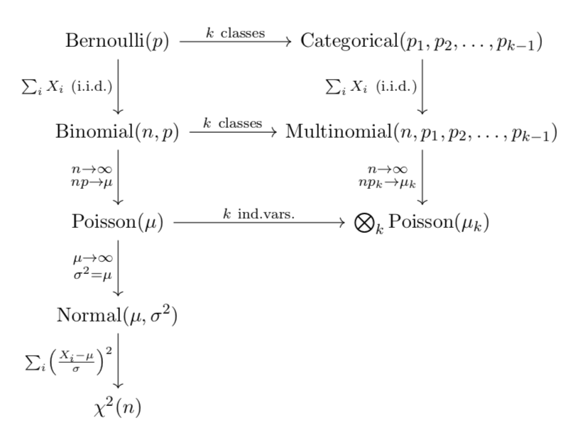
3.3.2.2 Normal/Gaussian distribution
\[ N(x \,|\, \mu, \sigma^2) = \frac{1}{\sqrt{2\,\pi\:\sigma^2}} \: \exp\left(\frac{-(x-\mu)^2}{2\,\sigma^2}\right) \]
and in \(k\) dimensions:
\[ N(\vec{x} \,|\, \vec{\mu}, \boldsymbol{\Sigma}) = (2 \pi)^{-k/2}\:\left|\boldsymbol{\Sigma}\right|^{-1/2} \: \exp\left(\frac{-1}{2}\:(\vec{x}-\vec{\mu})^\intercal \:\boldsymbol{\Sigma}^{-1}\:(\vec{x}-\vec{\mu})\right) \]
where \(\boldsymbol{\Sigma}\) is the covariance matrix of the distribution (defined in eq. 3.2).
3.3.3 Central limit theorem
Let \(X_{1}\), \(X_{2}\), … , \(X_{n}\) be a random sample drawn from any distribution with a finite mean \(\mu\) and variance \(\sigma^{2}\). As \(n \rightarrow \infty\), the distribution of
\[ \frac{\bar{X} - \mu}{\sigma/\sqrt{n}} \sim N(0, 1) \]
- \(\chi^2\) distribution
- Univariate distribution relationships
47 Leemis & McQueston (2008).
- The exponential family of distributions are maximum entropy distributions.
3.3.4 Mixture models
- Gaussian mixture models (GMM)
- Marked poisson
- pyhf model description
- HistFactory 48
48 Cranmer, K. et al. (2012).
3.4 Point estimation and confidence intervals
3.4.1 Inverse problems
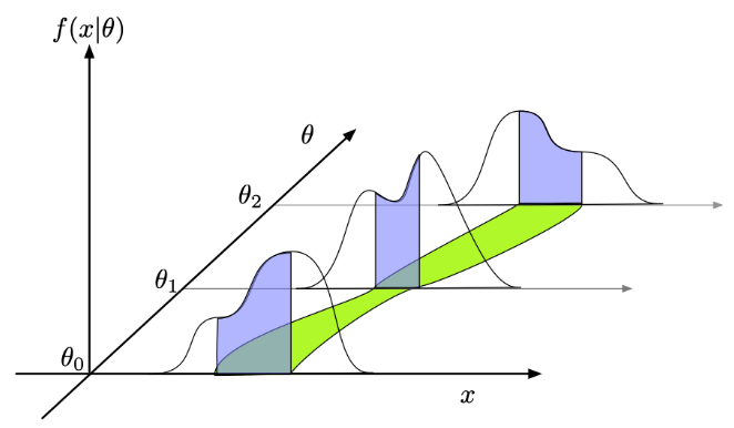
Recall that in the context of parametric models of data, \(x_i\) the pdf of which is modeled by a function, \(f(x_i ; \theta_j)\) with parameters, \(\theta_j\). In a statistical inverse problem, the goal is to infer values of the model parameters, \(\theta_j\) given some finite set of data, \(\{x_i\}\) sampled from a probability density, \(f(x_i; \theta_j)\) that models the data reasonably well 49.
49 This assumption that the model models the data “reasonably” well reflects that to the degree required by your analysis, the important features of the data match well within the systematic uncertainties parametrized within the model. If the model is incomplete because it is missing an important feature of the data, then this is the “ugly” (class-3) error in the Sinervo classification of systematic uncertainties.
- Inverse problem
- Inverse probability (Fisher)
- Statistical inference
- See also: Structural realism
- Estimators
- Regression
- Accuracy vs precision 50
3.4.2 Bias and variance
The bias of an estimator, \(\hat\theta\), is defined as
\[ \mathrm{Bias}(\hat{\theta}) \equiv \mathbb{E}(\hat{\theta} - \theta) = \int dx \: P(x|\theta) \: (\hat{\theta} - \theta) \]
The mean squared error (MSE) of an estimator has a similar formula to variance (eq. 3.1) except that instead of quantifying the square of the difference of the estimator and its expected value, the MSE uses the square of the difference of the estimator and the true parameter:
\[ \mathrm{MSE}(\hat{\theta}) \equiv \mathbb{E}((\hat{\theta} - \theta)^2) \]
The MSE of an estimator can be related to its bias and its variance by the following proof:
\[ \begin{align} \mathrm{MSE}(\hat{\theta}) &= \mathbb{E}(\hat{\theta}^2 - 2 \: \hat{\theta} \: \theta + \theta^2) \\ &= \mathbb{E}(\hat{\theta}^2) - 2 \: \mathbb{E}(\hat{\theta}) \: \theta + \theta^2 \end{align} \]
noting that
\[ \mathrm{Var}(\hat{\theta}) = \mathbb{E}(\hat{\theta}^2) - \mathbb{E}(\hat{\theta})^2 \]
and
\[ \begin{align} \mathrm{Bias}(\hat{\theta})^2 &= \mathbb{E}(\hat{\theta} - \theta)^2 \\ &= \mathbb{E}(\hat{\theta})^2 - 2 \: \mathbb{E}(\hat{\theta}) \: \theta + \theta^2 \end{align} \]
we see that MSE is equivalent to
\[ \mathrm{MSE}(\hat{\theta}) = \mathrm{Var}(\hat{\theta}) + \mathrm{Bias}(\hat{\theta})^2 \]
For an unbiased estimator, the MSE is the variance of the estimator.
TODO:
- Note the discussion of the bias-variance tradeoff by Cranmer.
- Note the new deep learning view. See Deep learning.
See also:
3.4.3 Maximum likelihood estimation
A maximum likelihood estimator (MLE) was first used by Fisher. 51
51 Aldrich (1997).
\[\hat{\theta} \equiv \underset{\theta}{\mathrm{argmax}} \: \mathrm{log} \: L(\theta) \]
Maximizing \(\mathrm{log} \: L(\theta)\) is equivalent to maximizing \(L(\theta)\), and the former is more convenient because for data that are independent and identically distributed (i.i.d.) the joint likelihood can be factored into a product of individual measurements:
\[ L(\theta) = \prod_i L(\theta|x_i) = \prod_i P(x_i|\theta) \]
and taking the log of the product makes it a sum:
\[ \mathrm{log} \: L(\theta) = \sum_i \mathrm{log} \: L(\theta|x_i) = \sum_i \mathrm{log} \: P(x_i|\theta) \]
Maximizing \(\mathrm{log} \: L(\theta)\) is also equivalent to minimizing \(-\mathrm{log} \: L(\theta)\), the negative log-likelihood (NLL). For distributions that are i.i.d.,
\[ \mathrm{NLL} \equiv - \log L = - \log \prod_i L_i = - \sum_i \log L_i = \sum_i \mathrm{NLL}_i \]
3.4.3.1 Invariance of likelihoods under reparametrization
- Likelihoods are invariant under reparametrization. 52
- Bayesian posteriors are not invariant in general.
52 F. James (2006), p. 234.
See also:
3.4.3.2 Ordinary least squares
3.4.4 Variance of MLEs
- Taylor expansion of a likelihood near its maximum
- Cramér-Rao bound 55
- Define efficiency of an estimator.
- Common formula for variance of unbiased and efficient estimators
- Proof in Rice 56
- Cranmer: Cramér-Rao bound
- Nielsen, F. (2013). Cramer-Rao lower bound and information geometry. 57
- Under some reasonable conditions, one can show that MLEs are efficient and unbiased. TODO: find ref.
- Fisher information matrix
- “is the key part of the proof of Wilks’ theorem, which allows confidence region estimates for maximum likelihood estimation (for those conditions for which it applies) without needing the Likelihood Principle.”
- Confidence intervals
- Variance of MLEs
- Wilks’s theorem
- Method of \(\Delta\chi^2\) or \(\Delta{}L\)
- Frequentist confidence intervals (e.g. at 95% CL)
- Cowan 58
- Likelihood need not be Gaussian 59
- Minos method in particle physics in MINUIT 60
- See slides for my talk: Primer on statistics: MLE, Confidence Intervals, and Hypothesis Testing
- Asymptotics
- See Asymptotics.
56 Rice (2007), p. 300–2.
57 Nielsen (2013).
58 Cowan (1998), p. 130-5.
59 F. James (2006), p. 234.
60 F. James & Roos (1975).
- Common error bars
- Poisson error bars
- Gaussian approximation: \(\sqrt{n}\)
- Wilson-Hilferty approximation
- Binomial error bars
- Error on efficiency or proportion
- See: Statistical classification
- Poisson error bars
- More on confidence intervals
- Loh, W.Y. (1987). Calibrating confidence coefficients. 61
- Discussion
- Wainer, H. (2007). The most dangerous equation. (de Moivre’s equation for variance of means) 62
- Misc
- Karhunen-Loève eigenvalue problems in cosmology: How should we tackle large data sets? 63
3.4.5 Bayesian credibility intervals
- Inverse problem to find a posterior probability distribution.
- Maximum a posteriori estimation (MAP)
- Prior sensitivity
- Betancourt, M. (2018). Towards a principled Bayesian workflow - ipynb
- Not invariant to reparametrization in general
- Jeffreys priors are
- TODO: James
3.4.6 Uncertainty on measuring an efficiency
- Binomial proportion confidence interval
- Normal/Gaussian/Wald interval
- Wilson score interval
- Clopper-Pearson interval (1934) 64
- Agresti-Coull interval (1998) 65
- Rule of three (1983) 66
- Review by Brown, Cai, & DasGupta (2001) 67
- Casadei, D. (2012). Estimating the selection efficiency. 68
- Precision vs recall for classification, again
- Classification and logistic regression
- See also:
- Logistic regression in the section on Classical machine learning.
- Clustering in the section on Classical machine learning.
3.4.7 Examples
- Some sample mean
- Bayesian lighthouse
- Measuring an efficiency
- Some HEP fit
3.5 Statistical hypothesis testing
3.5.1 Null hypothesis significance testing
- Karl Pearson observing how rare sequences of roulette spins are
- Null hypothesis significance testing (NHST)
- goodness of fit
- Fisher
Fisher:
3.5.2 Neyman-Pearson theory
3.5.2.1 Introduction
- probes an alternative hypothesis 70
- Type-1 and type-2 errors
- Power and confidence
- Cohen, J. (1992). A power primer. 71
- Cranmer, K. (2020). Thumbnail of LHC statistical procedures.
- ATLAS and CMS Collaborations. (2011). Procedure for the LHC Higgs boson search combination in Summer 2011. 72
- Cowan, G., Cranmer, K., Gross, E., & Vitells, O. (2011). Asymptotic formulae for likelihood-based tests of new physics. 73
70 Goodman (1999a). p. 998.
71 J. Cohen (1992).
72 ATLAS and CMS Collaborations (2011).
73 Cowan, Cranmer, Gross, & Vitells (2011).
See also:
3.5.2.2 Neyman-Pearson lemma
Neyman-Pearson lemma: 74
74 Neyman & Pearson (1933).
For a fixed signal efficiency, \(1-\alpha\), the selection that corresponds to the lowest possible misidentification probability, \(\beta\), is given by
\[ \frac{L(H_1)}{L(H_0)} > k_{\alpha} \]
where \(k_{\alpha}\) is the cut value required to achieve a type-1 error rate of \(\alpha\).
Neyman-Pearson test statistic:
\[ q_\mathrm{NP} = - 2 \ln \frac{L(H_1)}{L(H_0)} \]
Profile likelihood ratio:
\[ \lambda(\mu) = \frac{ L(\mu, \hat{\theta}_\mu) }{ L(\hat{\mu}, \hat{\theta}) } \]
where \(\hat{\theta}\) is the (unconditional) maximum-likelihood estimator that maximizes \(L\), while \(\hat{\theta}_\mu\) is the conditional maximum-likelihood estimator that maximizes \(L\) for a specified signal strength, \(\mu\), and \(\theta\) as a vector includes all other parameters of interest and nuisance parameters.
3.5.2.3 Neyman construction
Cranmer: Neyman construction.
TODO: fix
\[ q = - 2 \ln \frac{L(\mu\,s + b)}{L(b)} \]
3.5.2.4 Flip-flopping
- Flip-flopping and Feldman-Cousins confidence intervals 75
75 Feldman & Cousins (1998).
3.5.3 p-values and significance
- \(p\)-values and significance 76
- Coverage
- Fisherian vs Neyman-Pearson \(p\)-values
Cowan et al. define a \(p\)-value as
a probability, under assumption of \(H\), of finding data of equal or greater incompatibility with the predictions of \(H\). 77
77 Cowan et al. (2011), p. 2–3.
Also:
It should be emphasized that in an actual scientific context, rejecting the background-only hypothesis in a statistical sense is only part of discovering a new phenomenon. One’s degree of belief that a new process is present will depend in general on other factors as well, such as the plausibility of the new signal hypothesis and the degree to which it can describe the data. Here, however, we only consider the task of determining the \(p\)-value of the background-only hypothesis; if it is found below a specified threshold, we regard this as “discovery”. 78
78 Cowan et al. (2011), p. 3.
3.5.3.1 Uppper limits
- Cousins, R.D. & Highland, V.L. (1992). Incorporating systematic uncertainties into an upper limit. 79
79 Cousins & Highland (1992).
3.5.3.2 CLs method
3.5.4 Asymptotics
- Analytic variance of the likelihood-ratio of gaussians: \(\chi^2\)
- Pearson \(\chi^2\)-test
- Wilks 83
- Under the null hypothesis, \(-2 \ln(\lambda) \sim \chi^{2}_{k}\), where \(k\), the degrees of freedom for the \(\chi^{2}\) distribution is the number of parameters of interest (including signal strength) in the signal model but not in the null hypothesis background model.
- Wald 84
- Wald generalized the work of Wilks for the case of testing some nonzero signal for exclusion, showing \(-2 \ln(\lambda) \approx (\hat{\theta} - \theta)^\intercal V^{-1} (\hat{\theta} - \theta) \sim \mathrm{noncentral}\:\chi^{2}_{k}\).
- In the simplest case where there is only one parameter of interest (the signal strength, \(\mu\)), then \(-2 \ln(\lambda) \approx \frac{ (\hat{\mu} - \mu)^{2} }{ \sigma^2 } \sim \mathrm{noncentral}\:\chi^{2}_{1}\).
- Cowan, G., Cranmer, K., Gross, E., & Vitells, O. (2011). Asymptotic formulae for likelihood-based tests of new physics. 85
- Wald approximation
- Asimov dataset
- Talk by Armbruster: Asymptotic formulae (2013).
- Cowan, G., Cranmer, K., Gross, E., & Vitells, O. (2012). Asymptotic distribution for two-sided tests with lower and upper boundaries on the parameter of interest. 86
- Bhattiprolu, P.N., Martin, S.P., & Wells, J.D. (2020). Criteria for projected discovery and exclusion sensitivities of counting experiments. 87
3.5.5 Student’s t-test
- Student’s t-test
- ANOVA
- A/B-testing
3.5.6 Decision theory
- Suppes, P. (1961). The philosophical relevance of decision theory. The Journal of Philosophy, 58, 605–614. http://www.jstor.org/stable/2023536
- Frequentist vs bayesian decision theory 88
- Goodman, S.N. (1999). Toward evidence-based medical statistics 2: The Bayes factor. 89
Support for using Bayes factors:
which properly separates issues of long-run behavior from evidential strength and allows the integration of background knowledge with statistical findings. 90
90 Goodman (1999a). p. 995.
See also:
3.5.7 Examples
- Difference of two means: \(t\)-test
- A/B-testing
- New physics
3.6 Uncertainty quantification
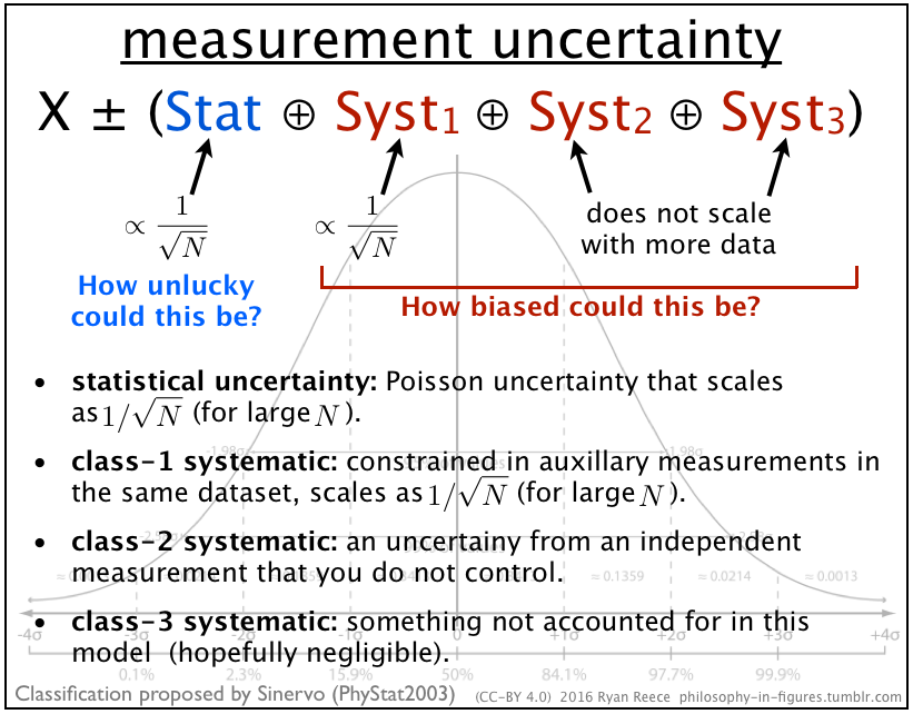
3.6.1 Sinervo classification of systematic uncertainties
- Class-1, class-2, and class-3 systematic uncertanties (good, bad, ugly), Classification by Pekka Sinervo (PhyStat2003) 91
- Not to be confused with type-1 and type-2 errors in Neyman-Pearson theory
- Heinrich, J. & Lyons, L. (2007). Systematic errors. 92
- Caldeira & Nord 93
Lyons:
In analyses involving enough data to achieve reasonable statistical accuracy, considerably more effort is devoted to assessing the systematic error than to determining the parameter of interest and its statistical error. 94
94 Lyons (2008), p. 890.
- Poincaré’s three levels of ignorance
3.6.2 Profile likelihoods
- Profiling and the profile likelihood
- Importance of Wald and Cowan et al.
- hybrid Bayesian-frequentist method
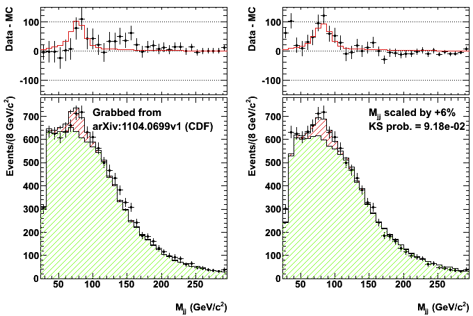
3.6.3 Examples of poor estimates of systematic uncertanties
- Unaccounted-for effects
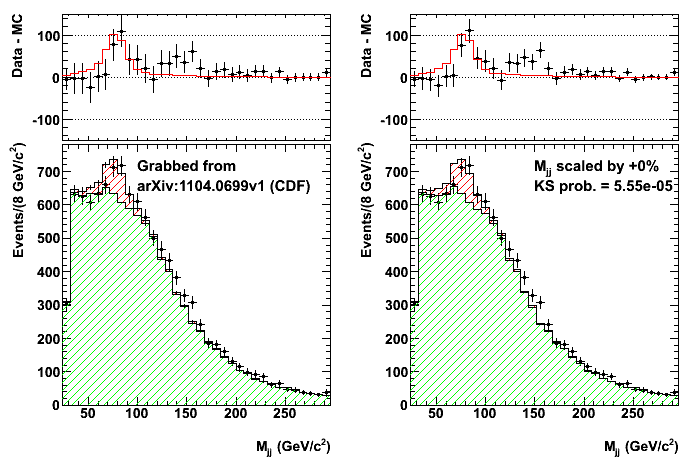
- CDF \(Wjj\) bump
- Phys.Rev.Lett.106:171801 (2011) / arxiv:1104.0699
- Invariant mass distribution of jet pairs produced in association with a \(W\) boson in \(p\bar{p}\) collisions at \(\sqrt{s}\) = 1.96 TeV
- Dorigo, T. (2011). The jet energy scale as an explanation of the CDF signal.
- OPERA. (2011). Faster-than-light neutrinos.
- BICEP2 claimed evidence of B-modes in the CMB as evidence of cosmic inflation without accounting for cosmic dust.
3.6.4 Conformal prediction
- Conformal prediction
- Gammerman, A., Vovk, V., & Vapnik, V. (1998). Learning by transduction. 95
95 Gammerman, Vovk, & Vapnik (1998).
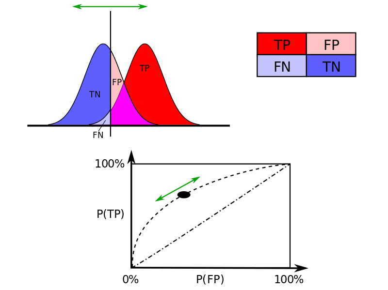
3.7 Statistical classification
3.7.1 Introduction
- Precision vs recall
- Recall is sensitivity
- Sensitivity vs specificity
- Accuracy
3.7.2 Examples
- TODO
See also:
3.8 Causal inference
3.8.1 Introduction
- Rubin, D. B. (1974). Estimating causal effects of treatments in randomized and nonrandomized studies. 96
- Lewis, D. (1981). Causal decision theory. 97
- Pearl, J. (2018). The Book of Why: The new science of cause and effect. 98
- Bareinboim, E., Correa, J.D., Ibeling, D., & Icard, T. (2021). On Pearl’s hierarchy and the foundations of causal inference. 99
See also:
3.8.2 Causal models
- Structural Causal Model (SCM)
- Pearl, J. (2009). Causal inference in statistics: An overview. 100
- Robins, J.M. & Wasserman, L. (1999). On the impossibility of inferring causation from association without background knowledge. 101
- Peters, J., Janzing, D., & Schölkopf, B. (2017). Elements of Causal Inference. 102
- Lundberg, I., Johnson, R., & Stewart, B.M. (2021). What is your estimand? Defining the target quantity connects statistical evidence to theory. 103
3.8.3 Counterfactuals
- Counterfactuals
- Regret
- Interventionist conception of causation
- Ismael, J. (2023). Reflections on the asymmetry of causation. 104
- Chevalley, M., Schwab, P., & Mehrjou, A. (2024). Deriving causal order from single-variable interventions: Guarantees & algorithm. 105
3.9 Exploratory data analysis
3.9.1 Introduction
- William Playfair (1759-1823)
- Father of statistical graphics
- John Tukey (1915-2000)
- Exploratory data analysis
- Exploratory Data Analysis (1977) 106
106 Tukey (1977).
3.9.2 Look-elsewhere effect
- Look-elsewhere effect (LEE)
- AKA File-drawer effect
- Stopping rules
- validation dataset
- statistical issues, violates the likelihood principle
3.9.3 Archiving and data science
- “Data science”
- Data collection, quality, analysis, archival, and reinterpretation
- Scientific research and big data
- Reproducible an reinterpretable
- RECAST
- Chen, X. et al. (2018). Open is not enough. 107
107 Chen, X. et al. (2018).
3.10 “Statistics Wars”
3.10.1 Introduction
Cranmer:
Bayes’s theorem is a theorem, so there’s no debating it. It is not the case that Frequentists dispute whether Bayes’s theorem is true. The debate is whether the necessary probabilities exist in the first place. If one can define the joint probability \(P (A, B)\) in a frequentist way, then a Frequentist is perfectly happy using Bayes theorem. Thus, the debate starts at the very definition of probability. 110
110 Cranmer (2015), p. 6.
Neyman:
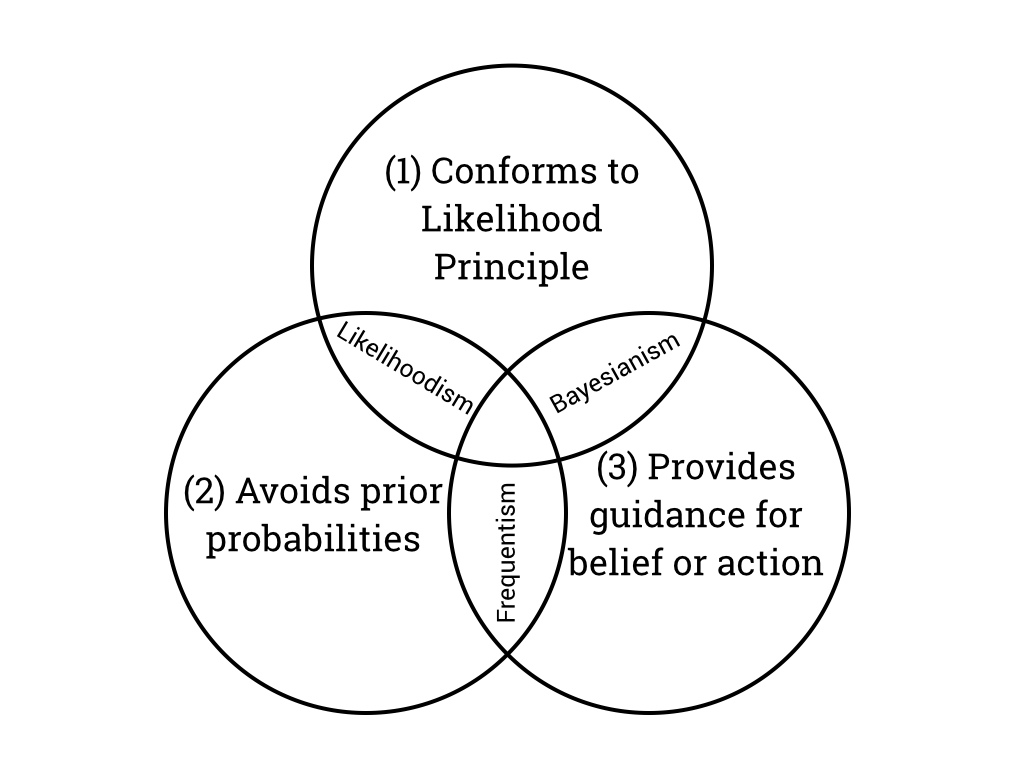
3.10.2 Likelihood principle
- Likelihood principle
- The likelihood principle is the proposition that, given a statistical model and a data sample, all the evidence relevant to model parameters is contained in the likelihood function.
- The history of likelihood 113
- Allan Birnbaum proved that the likelihood principle follows from two more primitive and seemingly reasonable principles, the conditionality principle and the sufficiency principle. 114
- Hacking identified the “law of likelihood”. 115
- Berger & Wolpert. (1988). The Likelihood Principle. 116
O’Hagan:
The first key argument in favour of the Bayesian approach can be called the axiomatic argument. We can formulate systems of axioms of good inference, and under some persuasive axiom systems it can be proved that Bayesian inference is a consequence of adopting any of these systems… If one adopts two principles known as ancillarity and sufficiency principles, then under some statement of these principles it follows that one must adopt another known as the likelihood principle. Bayesian inference conforms to the likelihood principle whereas classical inference does not. Classical procedures regularly violate the likelihood principle or one or more of the other axioms of good inference. There are no such arguments in favour of classical inference. 117
117 O’Hagan (2010), p. 17–18.
- Gandenberger
- “A new proof of the likelihood principle” 118
- Thesis: Two Principles of Evidence and Their Implications for the Philosophy of Scientific Method (2015)
- gandenberger.org/research
- Do frequentist methods violate the likelihood principle?
- Criticisms:
- Evans 119
- Mayo 120
- Mayo: The law of likelihood and error statistics 121
- Mayo’s response to Hennig and Gandenberger
- Dawid, A.P. (2014). Discussion of “On the Birnbaum Argument for the Strong Likelihood Principle”. 122
- Likelihoodist statistics
Mayo:
Likelihoods are vital to all statistical accounts, but they are often misunderstood because the data are fixed and the hypothesis varies. Likelihoods of hypotheses should not be confused with their probabilities. … [T]he same phenomenon may be perfectly predicted or explained by two rival theories; so both theories are equally likely on the data, even though they cannot both be true. 123
123 Mayo (2019).
3.10.3 Discussion
Lyons:
Particle Physicists tend to favor a frequentist method. This is because we really do consider that our data are representative as samples drawn according to the model we are using (decay time distributions often are exponential; the counts in repeated time intervals do follow a Poisson distribution, etc.), and hence we want to use a statistical approach that allows the data “to speak for themselves,” rather than our analysis being dominated by our assumptions and beliefs, as embodied in Bayesian priors. 124
124 Lyons (2008), p. 891.
- Carnap
- Carnap, R. (1952). The Continuum of Inductive Methods. 125
- Carnap, R. (1960). Logical Foundations of Probability. 126
- Sznajder on the alleged evolution of Carnap’s views of inductive logic 127
- David Cox
- Ian Hacking
- Logic of Statistical Inference 128
- Neyman
- “Frequentist probability and frequentist statistics” 129
- Rozeboom
- Rozeboom, W.W. (1960). The fallacy of the null-hypothesis significance test. 130
- Meehl
- Meehl, P. E. (1978). Theoretical risks and tabular asterisks: Sir Karl, Sir Ronald, and the slow progress of soft psychology. 131
- Zech
- “Comparing statistical data to Monte Carlo simulation” 132
- Richard Royall
- Statistical Evidence: A likelihood paradigm 133
- Jim Berger
- “Could Fisher, Jeffreys, and Neyman have agreed on testing?” 134
- Kendall & Stuart
- “The fiducialist argument rests on the assumption that \(\mathrm{probability}_{2}\) can be converted into \(\mathrm{probability}_{1}\) by means of a pivoting operation.” 135
- Deborah Mayo
- “In defense of the Neyman-Pearson theory of confidence intervals” 136
- Concept of “Learning from error” in Error and the Growth of Experimental Knowledge 137
- “Severe testing as a basic concept in a Neyman-Pearson philosophy of induction” 138
- “Error statistics” 139
- Statistical Inference as Severe Testing 140
- Statistics Wars: Interview with Deborah Mayo - APA blog
- Review of SIST by Prasanta S. Bandyopadhyay
- LSE Research Seminar: Current Controversies in Phil Stat (May 21, 2020)
- Meeting 5 (June 18, 2020)
- Slides: The Statistics Wars and Their Casualties
- Andrew Gelman
- Confirmationist and falsificationist paradigms of science - Sept. 5, 2014
- Beyond subjective and objective in statistics 141
- Retire Statistical Significance: The discussion
- Exchange with Deborah Mayo on abandoning statistical significance
- Several reviews of SIST
- Larry Wasserman
- Kevin Murphy
- Greg Gandenberger
- An introduction to likelihoodist, bayesian, and frequentist methods (1/3)
- As Neyman and Pearson put it in their original presentation of the frequentist approach, “without hoping to know whether each separate hypothesis is true or false, we may search for rules to govern our behavior with regard to them, in the following which we insure that, in the long run of experience, we shall not too often be wrong” (1933, 291).
- An introduction to likelihoodist, bayesian, and frequentist methods (2/3)
- An introduction to likelihoodist, bayesian, and frequentist methods (3/3)
- An argument against likelihoodist methods as genuine alternatives to bayesian and frequentist methods
- “Why I am not a likelihoodist” 144
- Jon Wakefield
- Bayesian and Frequentist Regression Methods 145
- Efron & Hastie
- “Flaws in Frequentist Inference” 146
- Kruschke & Liddel 147
- Steinhardt, J. (2012). Beyond Bayesians and frequentists. 148
- VanderPlas, J. (2014). Frequentism and Bayesianism III: Confidence, credibility, and why frequentism and science do not mix.
- Kent, B. (2021). No, your confidence interval is not a worst-case analysis.
- Aubrey Clayton
- Clayton, A. (2021). Bernoulli’s Fallacy: Statistical Illogic and the Crisis of Modern Science. 149
- Wagenmakers, E.J. (2021). Review: Bernoulli’s Fallacy. 150
125 Carnap (1952).
126 Carnap (1960).
127 Sznajder (2018).
128 Hacking (1965).
129 Neyman (1977).
130 Rozeboom (1960).
131 Meehl (1978).
132 Zech (1995).
133 Royall (1997).
134 Berger (2003).
135 Stuart et al. (2010), p. 460.
136 Mayo (1981).
137 Mayo (1996).
138 Mayo & Spanos (2006).
139 Mayo & Spanos (2011).
140 Mayo (2018).
141 Gelman & Hennig (2017).
142 Murphy (2012), ch. 6.6.
143 Murphy (2022), p. 195–198.
144 Gandenberger (2016).
145 Wakefield (2013), ch. 4.
146 Efron & Hastie (2016), p. 30–36.
147 Kruschke & Liddell (2018).
148 Steinhardt (2012).
149 Clayton (2021).
150 Wagenmakers (2021).
Goodman:
The idea that the \(P\) value can play both of these roles is based on a fallacy: that an event can be viewed simultaneously both from a long-run and a short-run perspective. In the long-run perspective, which is error-based and deductive, we group the observed result together with other outcomes that might have occurred in hypothetical repetitions of the experiment. In the “short run” perspective, which is evidential and inductive, we try to evaluate the meaning of the observed result from a single experiment. If we could combine these perspectives, it would mean that inductive ends (drawing scientific conclusions) could be served with purely deductive methods (objective probability calculations). 151
151 Goodman (1999a). p. 999.
3.11 Replication crisis
3.11.1 Introduction
- Ioannidis, J.P. (2005). Why most published research findings are false. 152
152 Ioannidis (2005).
3.11.2 p-value controversy
- Wasserstein, R.L. & Lazar, N.A. (2016). The ASA’s statement on \(p\)-values: Context, process, and purpose. 153
- Wasserstein, R.L., Allen, L.S., & Lazar, N.A. (2019). Moving to a World Beyond “p<0.05”. 154
- Big names in statistics want to shake up much-maligned P value 155
- Hi-Phi Nation, episode 7
- Fisher:
153 Wasserstein & Lazar (2016).
154 Wasserstein, Allen, & Lazar (2019).
155 Benjamin, D.J. et al. (2017).
[N]o isolated experiment, however significant in itself, can suffice for the experimental demonstration of any natural phenomenon; for the “one chance in a million” will undoubtedly occur, with no less and no more than its appropriate frequency, however surprised we may be that it should occur to us. In order to assert that a natural phenomenon is experimentally demonstrable we need, not an isolated record, but a reliable method of procedure. In relation to the test of significance, we may say that a phenomenon is experimentally demonstrable when we know how to conduct an experiment which will rarely fail to give us a statistically significant result. 156
156 Fisher (1935), p. 13–14.
- Relationship to the LEE
- Tukey, John (1915-2000)
- Wasserman
- Rao & Lovric
- Rao, C.R. & Lovric, M.M. (2016). Testing point null hypothesis of a normal mean and the truth: 21st century perspective. 157
- Mayo
- “Les stats, c’est moi: We take that step here!”
- “Significance tests: Vitiated or vindicated by the replication crisis in psychology?” 158
- At long last! The ASA President’s Task Force Statement on Statistical Significance and Replicability
- Gorard & Gorard. (2016). What to do instead of significance testing. 159
- Vox: What a nerdy debate about p-values shows about science–and how to fix it
- Karen Kafadar: The Year in Review … And More to Come
- The JASA Reproducibility Guide
From “The ASA president’s task force statement on statistical significance and replicability”:
P-values are valid statistical measures that provide convenient conventions for communicating the uncertainty inherent in quantitative results. Indeed, P-values and significance tests are among the most studied and best understood statistical procedures in the statistics literature. They are important tools that have advanced science through their proper application. 160
160 Benjamini, Y. et al. (2021), p. 1.
More:
- Bassily, R., Nissim, K., Smith, A., Steinke, T., Stemmer, U., & Ullman, J. (2015). Algorithmic stability for adaptive data analysis. 161
161 Bassily, R. et al. (2015).
3.12 Classical machine learning
3.12.1 Introduction
- Classification vs regression
- Supervised and unsupervised learning
- Classification = supervised; clustering = unsupervised
- Hastie, Tibshirani, & Friedman 162
- Information Theory, Inference, and Learning 163
- Murphy, K.P. (2012). Machine Learning: A probabilistic perspective. MIT Press. 164
- Murphy, K.P. (2022). Probabilistic Machine Learning: An introduction. MIT Press. 165
- Shalev-Shwarz, S. & Ben-David, S. (2014). Understanding Machine Learning: From Theory to Algorithms. 166
- VC-dimension
3.12.2 History
- History of artificial intelligence
- Arthur Samuel (1901-1990)
- Dartmouth workshop (1956)
- McCarthy, J., Minsky, M.L., Rochester, N., & Shannon, C.E. (1955). A proposal for the Dartmouth Summer Research Project on Artificial Intelligence. 169
- Solomonoff, G. (2016). Ray Solomonoff and the Dartmouth Summer Research Project in Artificial Intelligence, 1956. 170
- Rudolf Carnap (1891-1970)
- Kardum, M. (2020). Rudolf Carnap–The grandfather of artificial neural networks: The influence of Carnap’s philosophy on Walter Pitts. 171
- Bright, L.K. (2022). Carnap’s contributions.
- McCulloch & Pitts
- McCulloch, W. & Pitts, W. (1943). A logical calculus of ideas immanent in nervous activity. 172
- Anderson, J.A. & Rosenfeld, E. (1998). Talking Nets: An oral history of neural networks. 173
- Gefter, A. (2015). The man who tried to redeem the world with logic.
- Perceptron
- Rosenblatt, F. (1961). Principles of Neurodynamics: Perceptrons and the Theory of Brain Mechanisms. 174
- Sompolinsky, H. (2013). Introduction: The Perceptron.
- Connectionist vs symbolic AI
- Minsky, M. & Papert, S. (1969). Perceptrons: An Introduction to Computational Geometry. 175
- AI Winter
- Cartwright, N. (2001). What is wrong with Bayes nets?. 176
169 McCarthy, Minsky, Rochester, & Shannon (1955).
170 Solomonoff (2016).
171 Kardum (2020).
172 McCulloch & Pitts (1943).
173 J. A. Anderson & Rosenfeld (1998).
174 Rosenblatt (1961).
175 Minsky & Papert (1969).
176 Cartwright (2001).
See also:
- Honorific reinterpretation of scientism
3.12.3 Logistic regression
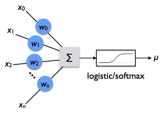
From a probabilistic point of view, 177 logistic regression can be derived from doing maximum likelihood estimation of a vector of model parameters, \(\vec{w}\), in a dot product with the input features, \(\vec{x}\), and squashed with a logistic function that yields the probability, \(\mu\), of a Bernoulli random variable, \(y \in \{0, 1\}\).
177 Murphy (2012), p. 21.
\[ p(y | \vec{x}, \vec{w}) = \mathrm{Ber}(y | \mu(\vec{x}, \vec{w})) = \mu(\vec{x}, \vec{w})^y \: (1-\mu(\vec{x}, \vec{w}))^{(1-y)} \]
The negative log-likelihood of multiple trials is
\[ \begin{align} \mathrm{NLL} &= - \sum_i \log p(y_i | \vec{x}_i, \vec{w}) \\ &= - \sum_i \log\left( \mu(\vec{x}_i, \vec{w})^{y_i} \: (1-\mu(\vec{x}_i, \vec{w}))^{(1-y_i)} \right) \\ &= - \sum_i \log\left( \mu_i^{y_i} \: (1-\mu_i)^{(1-y_i)} \right) \\ &= - \sum_i \big( y_i \, \log \mu_i + (1-y_i) \log(1-\mu_i) \big) \end{align} \]
which is the cross entropy loss. Note that the first term is non-zero only when the true target is \(y_i=1\), and similarly the second term is non-zero only when \(y_i=0\). 178 Therefore, we can reparametrize the target \(y_i\) in favor of \(t_{ki}\) that is one-hot in an index \(k\) over classes.
178 Note: Label smoothing is a regularization technique that smears the activation over other labels, but we don’t do that here.
\[ \mathrm{CEL} = \mathrm{NLL} = - \sum_i \sum_k \big( t_{ki} \, \log \mu_{ki} \big) \]
where
\[ t_{ki} = \begin{cases} 1 & \mathrm{if}\ (k = y_i = 0)\ \mathrm{or}\ (k = y_i = 1) \\ 0 & \mathrm{otherwise} \end{cases} \]
and
\[ \mu_{ki} = \begin{cases} 1-\mu_i & \mathrm{if}\ k = 0 \\ \mu_i & \mathrm{if}\ k =1 \end{cases} \]
This readily generalizes from binary classification to classification over many classes as we will discuss more below. Note that in the sum over classes, \(k\), only one term for the true class contributes.
\[ \mathrm{CEL} = - \left. \sum_i \log \mu_{ki} \right|_{k\ \mathrm{is\ such\ that}\ y_k=1} \tag{3.3}\]
Logistic regression uses the logit function 179, which is the logarithm of the odds—the ratio of the chance of success to failure. Let \(\mu\) be the probability of success in a Bernoulli trial, then the logit function is defined as
179 “Logit” was coined by Joseph Berkson (1899-1982).
\[ \mathrm{logit}(\mu) \equiv \log\left(\frac{\mu}{1-\mu}\right) \]
Logistic regression assumes that the logit function is a linear function of the explanatory variable, \(x\).
\[ \log\left(\frac{\mu}{1-\mu}\right) = \beta_0 + \beta_1 x \]
where \(\beta_0\) and \(\beta_1\) are trainable parameters. (TODO: Why would we assume this?) This can be generalized to a vector of multiple input variables, \(\vec{x}\), where the input vector has a 1 prepended to be its zeroth component in order to conveniently include the bias, \(\beta_0\), in a dot product.
\[ \vec{x} = (1, x_1, x_2, \ldots, x_n)^\intercal \]
\[ \vec{w} = (\beta_0, \beta_1, \beta_2, \ldots, \beta_n)^\intercal \]
\[ \log\left(\frac{\mu}{1-\mu}\right) = \vec{w}^\intercal \vec{x} \]
For the moment, let \(z \equiv \vec{w}^\intercal \vec{x}\). Exponentiating and solving for \(\mu\) gives
\[ \mu = \frac{ e^z }{ 1 + e^z } = \frac{ 1 }{ 1 + e^{-z} } \]
This function is called the logistic or sigmoid function.
\[ \mathrm{logistic}(z) \equiv \mathrm{sigm}(z) \equiv \frac{ 1 }{ 1 + e^{-z} } \]
Since we inverted the logit function by solving for \(\mu\), the inverse of the logit function is the logistic or sigmoid.
\[ \mathrm{logit}^{-1}(z) = \mathrm{logistic}(z) = \mathrm{sigm}(z) \]
And therefore,
\[ \mu = \mathrm{sigm}(z) = \mathrm{sigm}(\vec{w}^\intercal \vec{x}) \]
See also:
- Logistic regression
- Harlan, W.S. (2007). Bounded geometric growth: motivation for the logistic function.
- Heesch, D. A short intro to logistic regression.
- Roelants, P. (2019). Logistic classification with cross-entropy.
3.12.4 Softmax regression
Again, from a probabilistic point of view, we can derive the use of multi-class cross entropy loss by starting with the Bernoulli distribution, generalizing it to multiple classes (indexed by \(k\)) as
\[ p(y_k | \mu) = \mathrm{Cat}(y_k | \mu_k) = \prod_k {\mu_k}^{y_k} \]
which is the categorical or multinoulli distribution. The negative-log likelihood of multiple independent trials is
\[ \mathrm{NLL} = - \sum_i \log \left(\prod_k {\mu_{ki}}^{y_{ki}}\right) = - \sum_i \sum_k y_{ki} \: \log \mu_{ki} \]
Noting again that \(y_{ki} = 1\) only when \(k\) is the true class, and is 0 otherwise, this simplifies to eq. 3.3.
See also:
- Multinomial logistic regression
- McFadden 180
- Softmax is really a soft argmax. TODO: find ref.
- Softmax is not unique. There are other squashing functions. 181
- Roelants, P. (2019). Softmax classification with cross-entropy.
- Gradients from backprop through a softmax
- Goodfellow et al. point out that any negative log-likelihood is a cross entropy between the training data and the probability distribution predicted by the model. 182
3.12.5 Decision trees
- Freund, Y. & Schapire, R.E. (1997). A decision-theoretic generalization of on-line learning and an application to boosting. (AdaBoost) 183
- Chen, T. & Guestrin, C. (2016). Xgboost: A scalable tree boosting system. 184
- Aytekin, C. (2022). Neural networks are decision trees. 185
- Grinsztajn, L., Oyallon, E., & Varoquaux, G. (2022). Why do tree-based models still outperform deep learning on tabular data? 186
- Coadou, Y. (2022). Boosted decision trees. 187
3.12.6 Clustering
- unsupervised
- Gaussian Mixture Models (GMMs)
- Gaussian discriminant analysis
- \(\chi^2\)
- Generalized Linear Models (GLMs)
- Exponential family of PDFs
- Multinoulli \(\mathrm{Cat}(x|\mu)\)
- GLMs
- EM algorithm
- \(k\)-means
- Discussion
- Hartigan, J.A. (1985). Statistical theory in clustering. 188
- Clustering high-dimensional data
- t-distributed stochastic neighbor embedding (t-SNE)
- Slonim, N., Atwal, G.S., Tkacik, G. & Bialek, W. (2005). Information-based clustering. 189
- Topological data analysis
- Dindin, M. (2018). TDA To Rule Them All: ToMATo Clustering.
- Relationship of clustering and autoencoding
- Olah, C. (2014). Neural networks, manifolds, and topology.
- Batson et al. (2021). Topological obstructions to autoencoding. 190
- “What are the true clusters?” 191
- Lauc, D. (2020). Machine learning and the philosophical problems of induction. 192
- Ronen, M., Finder, S.E., & Freifeld, O. (2022). DeepDPM: Deep clustering with an unknown number of clusters. 193
- Fang, Z. et al. (2022). Is out-of-distribution detection learnable?. 194
188 Hartigan (1985).
189 Slonim, Atwal, Tkacik, & Bialek (2005).
190 Batson, Haaf, Kahn, & Roberts (2021).
191 Hennig (2015).
192 Lauc (2020), p. 103–4.
193 Ronen, Finder, & Freifeld (2022).
194 Fang, Z. et al. (2022).
See also:
3.13 Deep learning
3.13.1 Introduction
- Early contributions
- Gardner, M.W. & Dorling, S.R. (1998). Artificial neural networks (the multilayer perceptron)–a review of applications in the atmospheric sciences. 195
- Schmidhuber, J. (2024). A Nobel prize for plagiarism. 196
- Conceptual reviews of deep learning
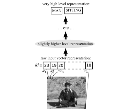
- Lower to higher level representations 197
- LeCun, Y., Bengio, Y., & Hinton, G. (2015). Review: Deep learning. 198
- Sutskever, I. (2015). A brief overview of deep learning. 199
- Deep Learning 200
- Kaplan, J. (2019). Notes on contemporary machine learning. 201
- Raissi, M. (2017). Deep learning tutorial.
- Arora, S. (2023). Theory of Deep Learning.
- Backpropagation
- Rumelhart, D.E., Hinton, G.E., & Williams, R.J. (1986). Learning representations by back-propagating errors. 202
- Amari, S. (1993). Backpropagation and stochastic gradient descent method. 203
- Schmidhuber’s Critique of Honda Prize for Dr. Hinton.
- Schmidhuber: Who invented backpropagation?
- Scmidhuber: The most cited neural networks all build on work done in my labs.
- LeCun, Y. & Bottou, L. (1998). Efficient BackProp. 204
- Pedagogy
- Bekman, S. (2023). Machine Learning Engineering Open Book.
- Labonne, M. (2023). Large Language Model Course.
- Microsoft. (2023). Generative AI for Beginners.
- Scardapane, S. (2024). Alice’s Adventures in a Differentiable Wonderland, Vol. I: A Tour of the Land. 205
- Grover, A. (2018). Notes on deep generative models.
- Practical guides
- Bottou, L. (1998). Stochastic gradient descent tricks. 206
- Bengio, Y. (2012). Practical recommendations for gradient-based training of deep architectures.
- Hao, L. et al. (2017). Visualizing the loss landscape of neural nets.
- Discussion
- Norvig, P. (2011). On Chomsky and the Two Cultures of Statistical Learning. 207
- Sutton, R. (2019). The bitter lesson. 208
- Frankle, J. & Carbin, M. (2018). The lottery ticket hypothesis: Finding sparse, trainable neural networks. 209
- AIMyths.com
195 Gardner & Dorling (1998).
196 Schmidhuber (2024).
197 Bengio (2009).
198 LeCun, Bengio, & Hinton (2015).
199 Sutskever (2015).
200 Goodfellow et al. (2016).
201 Kaplan, J. et al. (2019).
202 Rumelhart, Hinton, & Williams (1986).
203 Amari (1993).
204 LeCun & Bottou (1998).
205 Scardapane (2024).
206 Bottou (1998).
207 Norvig (2011).
208 Sutton (2019).
209 Frankle & Carbin (2018).
3.13.2 Gradient descent
\[ \hat{f} = \underset{f \in \mathcal{F}}{\mathrm{argmin}} \underset{x \sim \mathcal{X}}{\mathbb{E}} L(f, x) \]
The workhorse algorithm for optimizing (training) model parameters is gradient descent:
\[ \vec{w}[t+1] = \vec{w}[t] - \eta \frac{\partial L}{\partial \vec{w}}[t] \]
In Stochastic Gradient Descent (SGD), you chunk the training data into minibatches (AKA batches), \(\vec{x}_{bt}\), and take a gradient descent step with each minibatch:
\[ \vec{w}[t+1] = \vec{w}[t] - \frac{\eta}{m} \sum_{i=1}^m \frac{\partial L}{\partial \vec{w}}[\vec{x}_{bt}] \]
where
- \(t \in \mathbf{N}\) is the learning step number
- \(\eta\) is the learning rate
- \(m\) is the number of samples in a minibatch, called the batch size
- \(L\) is the loss function
- \(\frac{\partial L}{\partial \vec{w}}\) is the gradient
3.13.3 Deep double descent
- Bias and variance trade-off. See Bias and variance.
- MSE vs model capacity
Papers:
- Belkin, M., Hsu, D., Ma, S., & Mandal, S. (2019). Reconciling modern machine-learning practice and the classical bias-variance trade-off. 211
- Muthukumar, V., Vodrahalli, K., Subramanian, V., & Sahai, A. (2019). Harmless interpolation of noisy data in regression. 212
- Nakkiran, P., Kaplun, G., Bansal, Y., Yang, T., Barak, B., & Sutskever, I. (2019). Deep double descent: Where bigger models and more data hurt. 213
- Chang, X., Li, Y., Oymak, S., & Thrampoulidis, C. (2020). Provable benefits of overparameterization in model compression: From double descent to pruning neural networks. 214
- Holzmüller, D. (2020). On the universality of the double descent peak in ridgeless regression. 215
- Dar, Y., Muthukumar, V., & Baraniuk, R.G. (2021). A farewell to the bias-variance tradeoff? An overview of the theory of overparameterized machine learning. 216
- Balestriero, R., Pesenti, J., & LeCun, Y. (2021). Learning in high dimension always amounts to extrapolation. 217
- Belkin, M. (2021). Fit without fear: remarkable mathematical phenomena of deep learning through the prism of interpolation. 218
- Nagarajan, V. (2021). Explaining generalization in deep learning: progress and fundamental limits. 219
- Bach, F. (2022). Learning Theory from First Principles. 220
- Barak, B. (2022). The uneasy relationship between deep learning and (classical) statistics.
- Ghosh, N. & Belkin, M. (2022). A universal trade-off between the model size, test loss, and training loss of linear predictors. 221
- Singh, S.P., Lucchi, A., Hofmann, T., & Schölkopf, B. (2022). Phenomenology of double descent in finite-width neural networks. 222
- Hastie, T., Montanari, A., Rosset, S., & Tibshirani, R. J. (2022). Surprises in high-dimensional ridgeless least squares interpolation. 223
- Bubeck, S. & Sellke, M. (2023). A universal law of robustness via isoperimetry. 224
- Gamba, M., Englesson, E., Björkman, M., & Azizpour, H. (2022). Deep double descent via smooth interpolation. 225
- Schaeffer, R. et al. (2023). Double descent demystified: Identifying, interpreting & ablating the sources of a deep learning puzzle. 226
- Yang, T. & Suzuki, J. (2023). Dropout drops double descent. 227
- Maddox, W.J., Benton, G., & Wilson, A.G. (2023). Rethinking parameter counting in deep models: Effective dimensionality revisited. 228
211 Belkin, Hsu, Ma, & Mandal (2019).
212 Muthukumar, Vodrahalli, Subramanian, & Sahai (2019).
213 Nakkiran, P. et al. (2019).
214 Chang, Li, Oymak, & Thrampoulidis (2020).
215 Holzmüller (2020).
216 Dar, Muthukumar, & Baraniuk (2021).
217 Balestriero, Pesenti, & LeCun (2021).
218 Belkin (2021).
219 Nagarajan (2021).
220 Bach (2022), p. 225–230.
221 Ghosh & Belkin (2022).
222 Singh, Lucchi, Hofmann, & Schölkopf (2022).
223 Hastie, Montanari, Rosset, & Tibshirani (2022).
224 Bubeck & Sellke (2023).
225 Gamba, Englesson, Björkman, & Azizpour (2022).
226 Schaeffer, R. et al. (2023).
227 Yang & Suzuki (2023).
228 Maddox, Benton, & Wilson (2023).
Blogs:
- Hubinger, E. (2019). Understanding deep double descent. LessWrong.
- OpenAI. (2019). Deep double descent.
- Steinhardt, J. (2022). More is different for AI. 229
- Henighan, T. et al. (2023). Superposition, memorization, and double descent. 230
Twitter threads:
- Daniela Witten. (2020). Twitter thread: The bias-variance trade-off & double descent.
- François Fleuret. (2020). Twitter thread: The double descent with polynomial regression.
- adad8m. (2022). Twitter thread: The double descent with polynomial regression.
- Peyman Milanfar. (2022). Twitter thread: The perpetually undervalued least-squares.
- Pierre Ablin. (2023). Twitter thread: The double descent with polynomial regression.
3.13.4 Regularization
Regularization = any change we make to the training algorithm in order to reduce the generalization error but not the training error. 231
231 Mishra, D. (2020). Weight Decay == L2 Regularization?
Most common regularizations:
- L2 Regularization
- L1 Regularization
- Data Augmentation
- Dropout
- Early Stopping
Papers:
- Loshchilov, I. & Hutter, F. (2019). Decoupled weight decay regularization.
- Chen, S., Dobriban, E., & Lee, J. H. (2020). A group theoretic framework for data augmentation. 232
232 S. Chen, Dobriban, & Lee (2020).
3.13.5 Batch size vs learning rate
Papers:
- Keskar, N.S. et al. (2016). On large-batch training for deep learning: Generalization gap and sharp minima.
[L]arge-batch methods tend to converge to sharp minimizers of the training and testing functions—and as is well known—sharp minima lead to poorer generalization. In contrast, small-batch methods consistently converge to flat minimizers, and our experiments support a commonly held view that this is due to the inherent noise in the gradient estimation.
Hoffer, E. et al. (2017). Train longer, generalize better: closing the generalization gap in large batch training of neural networks.
- \(\eta \propto \sqrt{m}\)
Goyal, P. et al. (2017). Accurate large minibatch SGD: Training ImageNet in 1 hour.
- \(\eta \propto m\)
You, Y. et al. (2017). Large batch training of convolutional networks.
- Layer-wise Adaptive Rate Scaling (LARS)
You, Y. et al. (2017). ImageNet training in minutes.
- Layer-wise Adaptive Rate Scaling (LARS)
Jastrzebski, S. (2018). Three factors influencing minima in SGD.
- \(\eta \propto m\)
Smith, S.L. & Le, Q.V. (2018). A Bayesian Perspective on Generalization and Stochastic Gradient Descent.
Smith, S.L. et al. (2018). Don’t decay the learning rate, increase the batch size.
- \(m \propto \eta\)
Masters, D. & Luschi, C. (2018). Revisiting small batch training for deep neural networks.
This linear scaling rule has been widely adopted, e.g., in Krizhevsky (2014), Chen et al. (2016), Bottou et al. (2016), Smith et al. (2017) and Jastrzebski et al. (2017).
On the other hand, as shown in Hoffer et al. (2017), when \(m \ll M\), the covariance matrix of the weight update \(\mathrm{Cov(\eta \Delta\theta)}\) scales linearly with the quantity \(\eta^2/m\).
This implies that, adopting the linear scaling rule, an increase in the batch size would also result in a linear increase in the covariance matrix of the weight update \(\eta \Delta\theta\). Conversely, to keep the scaling of the covariance of the weight update vector \(\eta \Delta\theta\) constant would require scaling \(\eta\) with the square root of the batch size \(m\) (Krizhevsky, 2014; Hoffer et al., 2017).
Lin, T. et al. (2020). Don’t use large mini-batches, use local SGD.
- Post-local SGD.Golmant, N. et al. (2018). On the computational inefficiency of large batch sizes for stochastic gradient descent.
Scaling the learning rate as \(\eta \propto \sqrt{m}\) attempts to keep the weight increment length statistics constant, but the distance between SGD iterates is governed more by properties of the objective function than the ratio of learning rate to batch size. This rule has also been found to be empirically sub-optimal in various problem domains. … There does not seem to be a simple training heuristic to improve large batch performance in general.
- McCandlish, S. et al. (2018). An empirical model of large-batch training.
- Critical batch size
- Shallue, C.J. et al. (2018). Measuring the effects of data parallelism on neural network training.
In all cases, as the batch size grows, there is an initial period of perfect scaling (\(b\)-fold benefit, indicated with a dashed line on the plots) where the steps needed to achieve the error goal halves for each doubling of the batch size. However, for all problems, this is followed by a region of diminishing returns that eventually leads to a regime of maximal data parallelism where additional parallelism provides no benefit whatsoever.
- Jastrzebski, S. et al. (2018). Width of minima reached by stochastic gradient descent is influenced by learning rate to batch size ratio.
- \(\eta \propto m\)
We show this experimentally in Fig. 5, where similar learning dynamics and final performance can be observed when simultaneously multiplying the learning rate and batch size by a factor up to a certain limit.
- You, Y. et al. (2019). Large-batch training for LSTM and beyond.
- Warmup and use \(\eta \propto m\)
[W]e propose linear-epoch gradual-warmup approach in this paper. We call this approach Leg-Warmup (LEGW). LEGW enables a Sqrt Scaling scheme in practice and as a result we achieve much better performance than the previous Linear Scaling learning rate scheme. For the GNMT application (Seq2Seq) with LSTM, we are able to scale the batch size by a factor of 16 without losing accuracy and without tuning the hyper-parameters mentioned above.
- You, Y. et al. (2019). Large batch optimization for deep learning: Training BERT in 76 minutes.
- LARS and LAMB
- Zhang, G. et al. (2019). Which algorithmic choices matter at which batch sizes? Insights from a Noisy Quadratic Model.
Consistent with the empirical results of Shallue et al. (2018), each optimizer shows two distinct regimes: a small-batch (stochastic) regime with perfect linear scaling, and a large-batch (deterministic) regime insensitive to batch size. We call the phase transition between these regimes the critical batch size.
- Li, Y., Wei, C., & Ma, T. (2019). Towards explaining the regularization effect of initial large learning rate in training neural networks.
Our analysis reveals that more SGD noise, or larger learning rate, biases the model towards learning “generalizing” kernels rather than “memorizing” kernels.
Kaplan, J. et al. (2020). Scaling laws for neural language models.
Jastrzebski, S. et al. (2020). The break-even point on optimization trajectories of deep neural networks.
Blogs:
- Shen, K. (2018). Effect of batch size on training dynamics.
- Chang, D. (2020). Effect of batch size on neural net training.
3.13.6 Normalization
- BatchNorm
- LayerNorm, GroupNorm
- Online Normalization: Chiley, V. et al. (2019). Online normalization for training neural networks. 233
- Kiani, B., Balestriero, R., LeCun, Y., & Lloyd, S. (2022). projUNN: efficient method for training deep networks with unitary matrices. 234
- Huang, L. et al. (2020). Normalization techniques in training DNNs: Methodology, analysis and application. 235
3.13.7 Finetuning
- Hu, E.J. et al (2021). LoRA: Low-rank adaptation of large language models. 236
- Dettmers, T., Pagnoni, A., Holtzman, A., & Zettlemoyer, L. (2023). QLoRA: Efficient finetuning of quantized LLMs. 237
- Zhao, J. et al (2024). GaLore: Memory-efficient LLM training by gradient low-rank projection. 238
- Huh, M. et al. (2024). Training neural networks from scratch with parallel low-rank adapters. 239
3.13.8 Computer vision
- Computer Vision (CV)
- Fukushima: neocognitron 240
- LeNet-5
- LeCun, Y. (1989). Generalization and network design strategies.
- LeCun: OCR with backpropagation 241
- LeCun: LeNet-5 242
- Ciresan: MCDNN 243
- Krizhevsky, Sutskever, and Hinton: AlexNet 244
- VGG 245
- ResNet 246
- ResNet is performing a forward Euler discretisation of the ODE: \(\dot{x} = \sigma(F(x))\). 247
- MobileNet 248
- Neural ODEs 249
- EfficientNet 250
- VisionTransformer 251
- EfficientNetV2 252
- gMLP 253
- Dhariwal, P. & Nichol, A. (2021). Diffusion models beat GANs on image synthesis. 254
- Liu, Y. et al. (2021). A survey of visual transformers. 255
- Ingrosso, A. & Goldt, S. (2022). Data-driven emergence of convolutional structure in neural networks. 256
- Park, N. & Kim, S. (2022). How do vision transformers work? 257
- Zhao, Y. et al. (2023). DETRs beat YOLOs on real-time object detection. 258
- Nakkiran, P., Bradley, A., Zhou, H. & Advani, M. (2024). Step-by-step diffusion: An elementary tutorial. 259
240 Fukushima & Miyake (1982).
241 LeCun, Y. et al. (1989).
242 LeCun, Bottou, Bengio, & Haffner (1998).
243 Ciresan, Meier, Masci, & Schmidhuber (2012).
244 Krizhevsky, Sutskever, & Hinton (2012).
245 Simonyan & Zisserman (2014).
246 He, Zhang, Ren, & Sun (2015).
248 Howard, A.G. et al. (2017).
249 R. T. Q. Chen, Rubanova, Bettencourt, & Duvenaud (2018).
250 Tan & Le (2019).
251 Dosovitskiy, A. et al. (2020).
252 Tan & Le (2021).
253 H. Liu, Dai, So, & Le (2021).
254 Dhariwal & Nichol (2021).
255 Liu, Y. et al. (2021).
256 Ingrosso & Goldt (2022).
257 Park & Kim (2022).
258 Zhao, Y. et al. (2023).
259 Nakkiran, Bradley, Zhou, & Advani (2024).
Resources:
- Neptune.ai. (2021). Object detection algorithms and libraries.
- facebookresearch/vissl
- PyTorch Geometric (PyG)
3.13.9 Natural language processing
3.13.9.1 Introduction
- Natural Language Processing (NLP)
- History
- Firth, J.R. (1957): “You shall know a word by the company it keeps.” 260
- Nirenburg, S. (1996). Bar Hillel and Machine Translation: Then and Now. 261
- Hutchins, J. (2000). Yehoshua Bar-Hillel: A philosophers’ contribution to machine translation. 262
- Textbooks
- Jurafsky, D. & Martin, J.H. (2022). Speech and Language Processing: An introduction to natural language processing, computational linguistics, and speech recognition. 263
- Liu, Z., Lin, Y., & Sun, M. (2023). Representation Learning for Natural Language Processing. 264
3.13.9.2 word2vec
- Mikolov 265
- Julia Bazińska
- Olah, C. (2014). Deep learning, NLP, and representations.
- Alammar, J. (2019). The illustrated word2vec.
- Migdal, P. (2017). king - man + woman is queen; but why?
- Kun, J. (2018). A Programmer’s Introduction to Mathematics.
- Word vectors have semantic linear structure 266
- Ethayarajh, K. (2019). Word embedding analogies: Understanding King - Man + Woman = Queen.
- Allen, C. (2019). “Analogies Explained” … Explained.
3.13.9.3 RNNs
- RNNs and LSTMs
- Hochreiter, S. & Schmidhuber, J. (1997). Long short-term memory. 267
- Graves, A. (2013). Generating sequences with recurrent neural networks. 268
- Auto-regressive language modeling
- Olah, C. (2015). Understanding LSTM networks.
- Karpathy, A. (2015). The unreasonable effectiveness of recurrent neural networks.
Chain rule of language modeling (chain rule of probability):
\[ P(x_1, \ldots, x_T) = P(x_1, \ldots, x_{n-1}) \prod_{t=n}^{T} P(x_t | x_1 \ldots x_{t-1}) \]
or for the whole sequence:
\[ P(x_1, \ldots, x_T) = \prod_{t=1}^{T} P(x_t | x_1 \ldots x_{t-1}) \]
\[ = P(x_1) \: P(x_2 | x_1) \: P(x_3 | x_1 x_2) \: P(x_4 | x_1 x_2 x_3) \ldots \]
A language model (LM), predicts the next token given previous context. The output of the model is a vector of logits, which is given to a softmax to convert to probabilities for the next token.
\[ P(x_t | x_1 \ldots x_{t-1}) = \mathrm{softmax}\left( \mathrm{model}(x_1 \ldots x_{t-1}) \right) \]
Auto-regressive inference follows this chain rule. If done with greedy search:
\[ \hat{x}_t = \underset{x_t \in V}{\mathrm{argmax}} \: P(x_t | x_1 \ldots x_{t-1}) \]
Beam search:
- Beam search as used in NLP is described in Sutskever. 269
- Zhang, W. (1998). Complete anytime beam search. 270
- Zhou, R. & Hansen, E. A. (2005). Beam-stack search: Integrating backtracking with beam search. 271
- Collobert, R., Hannun, A., & Synnaeve, G. (2019). A fully differentiable beam search decoder. 272
269 Sutskever, Vinyals, & Le (2014), p. 4.
270 Zhang (1998).
271 Zhou & Hansen (2005).
272 Collobert, Hannun, & Synnaeve (2019).
Backpropagation through time (BPTT):
- Werbos, P.J. (1990). Backpropagation through time: what it does and how to do it. 273
273 Werbos (1990).
Neural Machine Translation (NMT):
3.13.9.4 Transformers
\[ \mathrm{attention}(Q, K, V) = \mathrm{softmax}\left(\frac{Q\, K^\intercal}{\sqrt{d_k}}\right) V \]
3.13.9.4.1 Attention and Transformers
- Transformer 278
- BERT 279
- Alammar, J. (2018). The illustrated BERT.
- Horev, R. (2018). BERT Explained: State of the art language model for NLP.
- Liu, Y. et al. (2019). RoBERTa: A robustly optimized BERT pretraining approach. 280
- Raffel, C. et al. (2019). Exploring the limits of transfer learning with a unified text-to-text transformer. (T5 model) 281
- Horan, C. (2021). 10 things you need to know about BERT and the transformer architecture that are reshaping the AI landscape.
- Video: What are transformer neural networks?
- Video: How to get meaning from text with language model BERT.
- ALBERT 282
- BART 283
- GPT-1 284, 2 285, 3 286
- Alammar, J. (2019). The illustrated GPT-2.
- Yang, Z. et al. (2019). XLNet: Generalized autoregressive pretraining for language understanding. 287
- Daily Nous: Philosophers On GPT-3.
- DeepMind’s blog posts for more details: AlphaFold1, AlphaFold2 (2020). Slides from the CASP14 conference are publicly available here.
- Joshi, C. (2020). Transformers are GNNs.
- Lakshmanamoorthy, R. (2020). A complete learning path to transformers (with guide to 23 architectures).
- Zaheer, M. et al. (2020). Big Bird: Transformers for longer sequences. 288
- Edelman, B.L., Goel, S., Kakade, S., & Zhang, C. (2021). Inductive biases and variable creation in self-attention mechanisms. 289
- Tay, Y., Dehghani, M., Bahri, D., & Metzler, D. (2022). Efficient transformers: A survey. 290
- Phuong, M. & Hutter, M. (2022). Formal algorithms for transformers. 291
- Chowdhery, A. et al. (2022). PaLM: Scaling language modeling with pathways. 292
- Ouyang, L. et al. (2022). Training language models to follow instructions with human feedback. (InstructGPT) 293
- OpenAI. (2022). Blog: ChatGPT: Optimizing Language Models for Dialogue.
- Wolfram, S. (2023). What is ChatGPT doing—and why does it work? 294
- GPT-4 295
- Mohamadi, S., Mujtaba, G., Le, N., Doretto, G., & Adjeroh, D.A. (2023). ChatGPT in the age of generative AI and large language models: A concise survey. 296
- Zhao, W.X. et al. (2023). A survey of large language models. 297
- 3Blue1Brown. (2024). Video: But what is a GPT? Visual intro to Transformers.
- Golovneva, O., Wang, T., Weston, J., & Sukhbaatar, S. (2024). Contextual position encoding: Learning to count what’s important. 298
- Apple. (2024). Apple Intelligence Foundation Language Models.
278 Vaswani, A. et al. (2017).
279 Devlin, Chang, Lee, & Toutanova (2018).
280 Liu, Y. et al. (2019).
281 Raffel, C. et al. (2019).
282 Lan, Z. et al. (2019).
283 Lewis, M. et al. (2019).
284 Radford, Narasimhan, Salimans, & Sutskever (2018).
285 Radford, A. et al. (2019).
286 Brown, T.B. et al. (2020).
287 Yang, Z. et al. (2019).
288 Zaheer, M. et al. (2020).
289 Edelman, Goel, Kakade, & Zhang (2021).
290 Tay, Dehghani, Bahri, & Metzler (2022).
291 Phuong & Hutter (2022).
292 Chowdhery, A. et al. (2022).
293 Ouyang, L. et al. (2022).
294 Wolfram (2023).
295 OpenAI (2023).
296 Mohamadi, S. et al. (2023).
297 Zhao, W.X. et al. (2023).
298 Golovneva, Wang, Weston, & Sukhbaatar (2024).
3.13.9.4.2 Computational complexity of transformers
- kipply (2022). Transformer inference arithmetic.
- Bahdanau, D. (2022). The FLOPs calculus of language model training.
- Sanger, A. (2023). Inference characteristics of Llama-2.
- Shenoy, V. & Kiely, P. (2023). A guide to LLM inference and performance.
- Anthony, Q., Biderman, S., & Schoelkopf, H. (2023). Transformer math 101.
3.13.9.4.3 Efficient transformers
- Dao, T., Fu, D.Y., Ermon, S., Rudra, A., & Ré, C. (2022). FlashAttention: Fast and memory-efficient exact attention with IO-awareness. 299
- Pope, R. et al. (2022). Efficiently scaling transformer inference.
- Dao, T. (2023). FlashAttention-2: Faster attention with better parallelism and work partitioning.
- Kim, S. et al. (2023). Full stack optimization of transformer inference: A survey.
- PyTorch. (2023). Accelerating generative AI with PyTorch II: GPT, Fast.
- Nvidia. (2023). Mastering LLM techniques: Inference optimization.
- Weng, L. (2023). Large transformer model inference optimization.
- Kwon, W. et al. (2023). Efficient memory management for large language model serving with PagedAttention.
- Zhang, L. (2023). Dissecting the runtime performance of the training, fine-tuning, and inference of large language models.
- Dettmers, T. (2023). Which GPU(s) to Get for Deep Learning: My Experience and Advice for Using GPUs in Deep Learning.
- Fu, Y. (2023). Towards 100x speedup: Full stack transformer inference optimization.
- Fu, Y. (2024). Challenges in deploying long-context transformers: A theoretical peak performance analysis.
- Fu, Y. et al. (2024). Data engineering for scaling language models to 128K context.
- Kwon, W. et al. (2023). Efficient memory management for large language model serving with PagedAttention. (vLLM)
- Shah, J. et al. (2024). FlashAttention-3: Fast and accurate attention with asynchrony and low-precision.
299 Dao, T. et al. (2022).
3.13.9.4.4 What comes after Transformers?
- Gu, A., Goel, K., & Ré, C. (2021). Efficiently modeling long sequences with structured state spaces. 300
- Merrill, W. & Sabharwal, A. (2022). The parallelism tradeoff: Limitations of log-precision transformers. 301
- Bulatov, A., Kuratov, Y., & Burtsev, M.S. (2022). Recurrent memory transformer. 302
- Raffel, C. (2023). A new alchemy: Language model development as a subfield?.
- Bulatov, A., Kuratov, Y., & Burtsev, M.S. (2023). Scaling transformer to 1M tokens and beyond with RMT. 303
- Bertsch, A., Alon, U., Neubig, G., & Gormley, M.R. (2023). Unlimiformer: Long-range transformers with unlimited length input. 304
- Mialon, G. et al. (2023). Augmented Language Models: a Survey. 305
- Peng, B. et al. (2023). RWKV: Reinventing RNNs for the Transformer Era. 306
- Sun, Y. et al. (2023). Retentive network: A successor to transformer for large language models. 307
- Gu, A. & Dao, T. (2023). Mamba: Linear-time sequence modeling with selective state spaces. 308
- Wang, H. et al. (2023). BitNet: Scaling 1-bit transformers for large language models. 309
- Ma, S. et al. (2024). The era of 1-bit LLMs: All large language models are in 1.58 bits. 310
- Ma, X. et al. (2024). Megalodon: Efficient LLM pretraining and inference with unlimited context length. 311
- Bhargava, A., Witkowski, C., Shah, M., & Thomson, M. (2023). What’s the magic word? A control theory of LLM prompting. 312
- Sun, Y. et al. (2024). Learning to (learn at test time): RNNs with expressive hidden states.
- Dao, T. & Gu, A. (2024). Transformers are SSMs: Generalized models and efficient algorithms through structured state space duality. 313
- Banerjee, S., Agarwal, A., & Singla, S. (2024). LLMs will always hallucinate, and we need to live with this. 314
- Jingyu Liu et al. (2025). TiDAR: Think in diffusion, talk in autoregression. 315
300 Gu, Goel, & Ré (2021).
301 Merrill & Sabharwal (2022).
302 Bulatov, Kuratov, & Burtsev (2022).
303 Bulatov, Kuratov, & Burtsev (2023).
304 Bertsch, Alon, Neubig, & Gormley (2023).
305 Mialon, G. et al. (2023).
306 Peng, B. et al. (2023).
307 Sun, Y. et al. (2023).
308 Gu & Dao (2023).
309 Wang, H. et al. (2023).
310 Ma, S. et al. (2024).
311 Ma, X. et al. (2024).
312 Bhargava, Witkowski, Shah, & Thomson (2023).
313 Dao & Gu (2024).
314 Banerjee, Agarwal, & Singla (2024).
315 Jingyu Liu et al (2025).
3.13.9.5 Evaluation methods
- Hendrycks, D. et al. (2020). Measuring Massive Multitask Language Understanding. (MMLU)
- Yue, X. et al. (2023). MMMU: A Massive Multi-discipline Multimodal Understanding and reasoning benchmark for expert AGI.
- Kim, J. et al. (2024). Evalverse: Unified and accessible library for large language model evaluation.
- Biderman, S. (2024). Lessons from the trenches on reproducible evaluation of language models.
- Stanford’s HELM Leaderboards
- Liang, P. et al. (2022). Holistic Evaluation of Language Models (HELM)
- Lee, T. et al. (2023). Holistic Evaluation of Text-To-Image Models (HEIM)
- github.com/stanford-crfm/helm
- EleutherAI/lm-evaluation-harness
- Srivastava, A. (2022). Beyond the Imitation Game: Quantifying and extrapolating the capabilities of language models.
- Suzgun, M. (2022). Challenging BIG-Bench Tasks and Whether Chain-of-Thought Can Solve Them.
- Wang, Y. (2024). MMLU-Pro: A More Robust and Challenging Multi-Task Language Understanding Benchmark.
3.13.9.6 Scaling laws in NLP
- Hestness, J. et al. (2017). Deep learning scaling is predictable, empirically. 316
- Church, K.W. & Hestness, J. (2019). Rationalism and empiricism in artificial intellegence: A survey of 25 years of evaluation [in NLP]. 317
- Kaplan, J. et al. (2020). Scaling laws for neural language models. 318
- Rae, J.W. et al. (2022). Scaling language models: Methods, analysis & insights from training Gopher. 319
- Hoffmann, J. et al. (2022). Training compute-optimal large language models (Chinchilla). 320
- Caballero, E., Gupta, K., Rish, I., & Krueger, D. (2022). Broken neural scaling laws. 321
- Constantin, S. (2023). “Scaling Laws” for AI and some implications.
- Muennighoff, N. et al. (2023). Scaling data-constrained language models. 322
- Pandey, R. (2024). gzip predicts data-dependent scaling laws. 323
- Bach, F. (2024). Scaling laws of optimization. 324
- Finzi, M. et al. (2025). Compute-optimal LLMs provably generalize better with scale. 325
3.13.9.7 Language understanding
- NLU
- Mahowald, K. et al. (2023). Dissociating language and thought in large language models: a cognitive perspective. 326
- Kosinski, M. (2023). Theory of mind may have spontaneously emerged in large language models. 327
- Chitra, T. & Prior, H. (2023). Do language models possess knowledge (soundness)?
- Shani, C., Jurafsky, D., LeCun, Y., et Shwartz-Ziv, R. (2025). From tokens to thoughts: How LLMs and humans trade compression for meaning. [^Shani2025]
See also:
3.13.9.8 Interpretability
- Grandmother cell
- Watson, D. & Floridi, L. (2019). The explanation game: A formal framework for interpretable machine learning. 328
- Anthropic. (2021). A mathematical framework for transformer circuits.
- Anthropic. (2022). In-context learning and induction heads.
- Gurnee, W. et al. (2023). Finding neurons in a haystack: Case studies with sparse probing. 329
- Meng, K., Bau, D., Andonian, A., & Belinkov, Y. (2023). Locating and editing factual associations in GPT. 330
- McDougall, C., Conmy, A., Rushing, C., McGrath, T., & Nanda, N. (2023). Copy suppression: Comprehensively understanding an attention head. 331
- Anthropic. (2025). On the biology of a large language model.
328 Watson & Floridi (2019).
329 Gurnee, W. et al. (2023).
330 Meng, Bau, Andonian, & Belinkov (2023).
331 McDougall, C. et al. (2023).
Linear probes:
- Alain, G. & Bengio, Y. (2016). Understanding intermediate layers using linear classifier probes. 332
- Belinkov, Y. (2022). Probing classifiers: Promises, shortcomings, and advances. 333
- Gurnee, W. & Tegmark, M. (2023). Language models represent space and time. 334
3.13.10 Reinforcement learning
- Reinforcement Learning (RL)
- Dynamic programming
- Bellman equation
- Backward induction
- John von Neumann & Oskar Morgenstern. (1944). Theory of Games and Economic Behavior.
Pedagogy:
- Sutton & Barto 335
- Deep Reinforcement Learning: A Brief Survey 336
- Cesa-Bianchi, N. & Lugosi, G. (2006). Prediction, Learning, and Games. 337
- OpenAI. (2018). Spinning Up.
335 Sutton & Barto (2018).
336 Arulkumaran, Deisenroth, Brundage, & Bharath (2017).
337 Cesa-Bianchi & Lugosi (2006).
Tutorials:
- RL course by David Silver
- RL course by Emma Brunskill
- DeepMind Reinforcement Learning Lecture Series 2021
More:
- List by OpenAI of key RL papers
- List of game AI codes by DATA Lab
- Xu, Z., van Hasselt, H., & Silver, D. (2018). Meta-gradient reinforcement learning. 338
- Chen, L. et al. (2021). Decision Transformer: Reinforcement learning via sequence modeling.
- Silver, D., Singh, S., Precup, D., & Sutton, R.S. (2024). Reward is enough. 339
- Javed, K. & Sutton, R.S. (2024). The big world hypothesis and its ramifications for artificial intelligence. 340
338 Xu, Hasselt, & Silver (2018).
339 Silver, Singh, Precup, & Sutton (2024).
340 Javed & Sutton (2024).
See also:
3.13.10.1 Q-learning
- Q-learning and DQN
- Uses the Markov Decision Process (MDP) framework
- The Bellman equation 341
- Q-learning is a values-based learning algorithm. Value based algorithms updates the value function based on an equation (particularly Bellman equation). Whereas the other type, policy-based estimates the value function with a greedy policy obtained from the last policy improvement (source: towardsdatascience.com).
- DQN masters Atari 342
3.13.10.2 AlphaZero
- AlphaGo Lee 343 → AlphaGo Zero 344 → AlphaZero 345
- OpenAI Five masters Dota2
- AlphaStar masters StarCraftII
- AlphaZero
- \(\pi(a|s)\) and \(V(s)\)
- Monte Carlo Tree Search (MCTS)
3.13.10.3 Regret minimization
Regret matching (RM)
- Hart, S. & Mas‐Colell, A. (2000). A simple adaptive procedure leading to correlated equilibrium. 346
346 Hart & Mas‐Colell (2000).
Consider a game like rock-paper-scissors, where there is only one action per round. Let \(v^{t}(a)\) be the value observed when playing action \(a\) on iteration \(t\).
TODO: explain that the entire rewards vector, \(v^{t}(a)\), over \(a\) is observable after the chosen action is played.
Let a strategy, \(\sigma^t\), be a probability distribution over actions, \(a \in A\). Then the value of a strategy, \(v^{t}(\sigma^{t})\), is the expectation of its value over actions.
\[ v^{t}(\sigma^{t}) = \sum_{a \in A} \sigma^{t}(a) \: v^{t}(a) \]
Regret, \(R^{T}\), measures how much better some sequence of strategies, \(\sigma'\), would do compared to the chosen sequence of strategies, \(\sigma = \{\sigma^1, \sigma^2, \ldots \sigma^T\}\).
\[ R^{T} \equiv \sum_{t=1}^{T} \left( v^{t}({\sigma'}^{t}) - v^{t}(\sigma^{t}) \right) \]
External regret, \(R^{T}(a)\), measures the regret of the chosen sequence of strategies versus a hypothetical stategy where action \(a\) is always chosen.
\[ R^{T}(a) \equiv \sum_{t=1}^{T} \left( v^{t}(a) - v^{t}(\sigma^{t}) \right) \]
Regret Matching (RM) is a rule to determine the strategy for the next iteration:
\[ \sigma^{t+1}(a) \equiv \frac{ R^{t}_{+}(a) }{ \sum_{b \in A} R^{t}_{+}(b) } \]
where \(R_{+} \equiv \mathrm{max}(R, 0)\).
At the end of training, the resulting recommended strategy with convergence bounds is not the final strategy used in training, \(\sigma^{T}\), but the average strategy over all time steps:
\[ \bar{\sigma}^{T}(a) = \frac{1}{T} \sum_{t=1}^{T} \sigma^{t}(a) \]
- TODO: explain the convergence of \(\bar{\sigma}^{t}\) to an \(\varepsilon\)-Nash equilibrium.
- Roughgarden, T. (2016). Twenty Lectures on Algorithmic Game Theory. 347
347 Roughgarden (2016).
Counterfactual regret minimization (CFR)
- CFR
- Zinkevich, M., Johanson, M., Bowling, M., & Piccione, C. (2007). Regret minimization in games with incomplete information. 348
- Counterfactual regret minimization (CFR) is an algorithm for extensive-form games that independently minimizes regret in each information set. 349
- “In other words, actions are selected in proportion to the amount of positive counterfactual regret for not playing that action.” 350
- CFR differs from traditional RL algorithms in that it does not try to maximize expected return. Instead, it minimizes exploitability. CFR does not use the MDP framework; instead, it uses extensive-form games (source: Quora).
- Johanson’s explanation on Quora.
- CFR+
- Tammelin, O. (2014). Solving large imperfect information games using CFR+. 351
- Tammelin, O., Burch, N., Johanson, M., & Bowling, M. (2015). Solving heads-up limit texas hold’em 352
- Burch, N., Moravcik, M., & Schmid, M. (2019). Revisiting CFR+ and alternating updates. 353
- Brown, N. & Sandholm, T. (2019). Solving imperfect-information games via discounted regret minimization. 354
- LCFR+ is worse than CFR+ or LCFR.
- Examples
348 Zinkevich, Johanson, Bowling, & Piccione (2007).
349 N. Brown (2020), p. 12.
350 Zinkevich et al. (2007), p. 4.
351 Tammelin (2014).
352 Tammelin, Burch, Johanson, & Bowling (2015).
353 Burch, Moravcik, & Schmid (2019).
354 N. Brown & Sandholm (2019a).
TODO: explain extensive-form games.
A finite extensive game with imperfect information has the following components: 355
- A finite set \(N\) of players. A finite set \(H\) of sequences, the possible histories of actions, such that the empty sequence is in \(H\) and every prefix of a sequence in \(H\) is also in \(H\). Define \(h \sqsubseteq h'\) to mean \(h\) is a prefix of \(h'\). \(Z \subseteq H\) are the terminal histories (those which are not a prefix of any other sequences). \(A(h) = \{a : ha \in H\}\) are the actions available after a non-terminal history, \(h \in H \backslash Z\).
- A function \(P\) that assigns to each non-terminal history a member of \(N \cup \{c\}\). \(P\) is the player function. \(P(h)\) is the player who takes an action after the history \(h\). If \(P(h) = c\) then chance determines the action taken after history \(h\).
- For each player \(i \in N \cup \{c\}\) a partition \(\mathcal{I}_i\) of \(\{h \in H : P (h) = i\}\) with the property that \(A(h) = A(h')\) whenever \(h\) and \(h'\) are in the same member of the partition. For \(I \in \mathcal{I}_i\) we denote by \(A(I_i)\) the set \(A(h)\) and by \(P(I_i)\) the player \(P(h)\) for any \(h \in I_i\) . \(\mathcal{I}_i\) is the information partition of player \(i\); a set \(I_i \in \mathcal{I}_i\) is an information set of player \(i\).
- A function \(f_c\) that associates with every information set \(I\) where \(P(I) = c\), a probability measure \(f_c(a|I)\) on \(A(h)\); \(f_c(a|I)\) is the probability that \(a\) occurs given some \(h \in I\), where each such probability measure is independent of every other such measure.
- For each player \(i \in N\) there is a utility function \(u_i\) from the terminal states \(Z\) to the reals \(\mathbb{R}\). If \(N = \{1, 2\}\) and \(u_1 = -u_2\), it is a zero-sum extensive game. Define \(\Delta_{u,i} \equiv \mathrm{max}_z \: u_i(z) - \mathrm{min}_z \: u_i(z)\) to be the range of utilities to player \(i\).
The player reach, \(\pi^{\sigma}_{i}(h)\), of a history \(h\) is the product of the probabilities for all agent \(i\) actions leading to \(h\). Formally, 356
356 N. Brown (2020), p. 6.
\[ \pi^{\sigma}_{i}(h) \equiv \prod_{h' \cdot a' \sqsubseteq h | P(h') = i} \sigma_{i}(h', a') \]
Due to perfect recall, any two histories in infoset \(I_i\) have the same player reach for player \(i\). Thus, we similarly define the player reach \(\pi^{\sigma}_{i}(I_i)\) of infoset \(I_i\) as
\[ \pi^{\sigma}_{i}(I_i) \equiv \prod_{ {I'}_{i} \cdot a' \sqsubseteq I_i | P(I_i) = i } \sigma_{i}({I'}_{i}, a') = \left.\pi^{\sigma}_{i}(h)\right|_{h \in I_i} \]
The external reach AKA opponent reach, \(\pi^{\sigma}_{-i}(h)\), of a history \(h\) is the contribution of chance and all other players than \(i\). Formally,
\[ \pi^{\sigma}_{-i}(h) \equiv \prod_{h' \cdot a' \sqsubseteq h | P(h') \neq i} \sigma_{i}(h', a') \]
We also define the external reach of an infoset as
\[ \pi^{\sigma}_{-i}(I_i) \equiv \sum_{h \in I_{i}} \pi^{\sigma}_{-i}(h) \]
The counterfactual value of an infoset \(I\) is the expected utility to player \(i\) given that \(I\) has been reached, weighted by the external reach of \(I\) for player \(i\). Formally, 357
357 N. Brown (2020), p. 12.
\[ v(I) = \sum_{h \in I} \pi^{\sigma}_{-i}(h) \sum_{z \in Z} \pi^{\sigma}(h, z) \: u_{i}(z) \]
The counterfactual value of an action, \(a\), is
\[ v(I, a) = \sum_{h \in I} \pi^{\sigma}_{-i}(h) \sum_{z \in Z} \pi^{\sigma}(h \cdot a, z) \: u_{i}(z) \]
Let’s consider the case where, like in NLHE, our two private hole cards each make a single unique history \(h\), and we form infosets with a single hand, so \(I=h\). Then
\[ v(h) = \pi^{\sigma}_{-i}(h) \sum_{z \in Z} \pi^{\sigma}(h, z) \: u_{i}(z) \]
making explicit the player reach and the external reach,
\[ v(h) = \pi^{\sigma}_{-i}(h) \sum_{z \in Z} \pi_{i}^{\sigma}(h, z) \: \pi_{-i}^{\sigma}(h, z) \: u_{i}(z) \]
At a leaf node where we finally calculate the rewards,
\[ v(z) = \pi^{\sigma}_{-i}(z) \: u_{i}(z) \]
TODO: explain CFR.
The instantaneous regret is
\[ r^{t}(I, a) = v^{\sigma^t}(I, a) - v^{\sigma^t}(I) \]
The (cummulative) counterfactual regret
\[ R^{t}(I, a) = \sum_{t=1}^{T} r^{t}(I, a) \]
Similar to the single-node game discussed above, eq. \(\eqref{eq:regret_matching}\), applying regret matching during training means to update strategies according to the following rule.
\[ \sigma^{t+1}(I, a) \equiv \frac{ R^{t}_{+}(I, a) }{ \sum_{b \in A} R^{t}_{+}(I, b) } \]
The average strategy is
\[ \bar{\sigma}^{T}(I, a) = \sum_{t=1}^{T} \frac{\pi^{t}_{i}(I) \: \sigma^{t}(I, a) }{\pi^{t}_{i}(I)} \]
Monte Carlo Counterfactual Regret Minimization (MCCFR)
- Lanctot, M. (2009). Monte Carlo sampling for regret minimization. 358
- Neller, T.W. & Lanctot, M. (2013). An introduction to counterfactual regret minimization. 359
- Vectorized and sampling variants
- Burch, N., Lanctot, M., Szafron, D., & Gibson, R. (2012). Efficient Monte Carlo counterfactual regret minimization in games with many player actions. 360
- Johanson, M., Bard, N., Lanctot, M., Gibson, R.G., & Bowling, M. (2012). Efficient Nash equilibrium approximation through Monte Carlo counterfactual regret minimization. 361
- Variants of chance sampling with single or vector opponent actions.
- Schmid, M. et al. (2019). Variance reduction in Monte Carlo counterfactual regret minimization (VR-MCCFR) for extensive form games using baselines. 362
- Li, H. et al. (2020). Regret minimization via novel vectorized sampling policies and exploration. 363
- Habara, K., Fukuda, E.H., & Yamashita, N. (2023). Convergence analysis and acceleration of the smoothing methods for solving extensive-form games. 364
- MCCFR Ph.D. theses
- Lanctot, M. (2013). Monte Carlo Sample and Regret Minimization for Equilibrium Computation and Decision-Making in Large Extensive Form Games. 365
- Gibson, R. (2014). Regret minimization in games and the development of champion multiplayer computer poker-playing agents. 366
- Johanson, M. (2016). Robust Strategies and Counter-Strategies: From Superhuman to Optimal Play. 367
- Burch, N. (2018). Time and Space: Why imperfect information games are hard. 368
- Horacek, M. (2022). Risk-Aversion in Algorithms for Poker. 369
358 Lanctot et al. (2009).
359 Neller & Lanctot (2013).
360 Burch, Lanctot, Szafron, & Gibson (2012).
361 Johanson, M. et al. (2012).
362 Schmid, M. et al. (2019).
363 Li, H. et al. (2020).
364 Habara, Fukuda, & Yamashita (2023).
365 Lanctot (2013).
366 Gibson (2014).
367 Johanson (2016).
368 Burch (2018).
369 Horacek (2022).
TODO: explain MCCFR.
External sampling MCCFR:
\[ \tilde{v}^{\sigma}_{i}(I) = \sum_{z \in Q} u_{i}(z) \: \pi^{\sigma}_{i}(z[I] \rightarrow z) \]
Best response and exploitability
Best response:
\[ \mathrm{BR}(\sigma_{-i}) = \underset{\sigma_{i}^{\prime}}{\mathrm{argmax}} \: u_{i}(\sigma_{i}^{\prime}, \sigma_{-i}) \]
TODO: Local Best Response (LBR). 370
370 Lisy & Bowling (2016), p. 2.
Exploitability:
\[ \varepsilon_{i}(\sigma) = u_{i}(\mathrm{BR}(\sigma_{-i}), \sigma_{-i}) - u_{i}(\sigma_{i}, \mathrm{BR}(\sigma_{i})) \]
NashConv 371 exploitability uses the convention:
371 See NashConv exploitability defined in Lanctot, M. et al. (2017).
\[ \varepsilon_{i}(\sigma) = u_{i}(\mathrm{BR}(\sigma_{-i}), \sigma_{-i}) - u_{i}(\sigma_{i}, \sigma_{-i}) \]
The average exploitability per player is
\[ \varepsilon(\sigma) = \frac{1}{n} \sum_{i}^{n} \varepsilon_{i}(\sigma) \]
Note that in zero-sum games, when summing over players, the second terms in NashConv sum to zero. 372
372 Timbers (2020), p. 3.
\[ \varepsilon(\sigma) = \frac{1}{n} \sum_{i}^{n} u_{i}(\mathrm{BR}(\sigma_{-i}), \sigma_{-i}) \]
In two-player games:
\[ \varepsilon(\sigma) = \frac{1}{2} \Big( u_{1}(\mathrm{BR}(\sigma_{2}), \sigma_{2}) + u_{2}(\sigma_{1}, \mathrm{BR}(\sigma_{1})) \Big) \]
- Johanson, M., Waugh, K., Bowling, M., & Zinkevich, M. (2011). Accelerating best response calculation in large extensive games. 373
- Evaluates range vs range rewards in \(O(n \log n)\) + \(O(n)\) instead of \(O(n^2)\).
- Ponsen, M., De Jong, S., & Lanctot, M. (2011). Computing approximate Nash equilibria and robust best-responses using sampling. 374
- Lisy, V. & Bowling, M. (2016). Equilibrium approximation quality of current no-limit poker bots. 375
- Timbers, F. (2020). Approximate exploitability: Learning a best response in large games. 376
3.13.10.4 Solving poker
- Simplified toy pokers
- Earlier poker work
- Billings, D., Davidson, A., Schaeffer, J., & Szafron, D. (2002). The challenge of poker. 379
- Billings, D. et al. (2003). Approximating game-theoretic optimal strategies for full-scale poker. 380
- Johanson, M. (2013). Measuring the size of large no-limit poker games. 381
- Claudico (2015) - Sandholm, T. et al. (CMU)
- Bowling, M., Burch, N., Johanson, M., & Tammelin, O. (2015). Heads-up limit hold’em poker is solved. 382
- CFR+
- Heinrich & Silver. (2016). Deep reinforcement learning from self play in imperfect-information games. 383
- Q-learning
- Moravcik, M. et al. (2017). DeepStack: Expert-level artificial intelligence in heads-up no-limit poker. 384
- Libratus
- Brown, N. & Sandholm, T. (2017). Safe and nested subgame solving for imperfect-information games. 385
- Adds test-time search/planning to just using precomputed policies.
- Brown, N. & Sandholm, T. (2018). Superhuman AI for heads-up no-limit poker: Libratus beats top professionals. 386
- bet and card abstraction
- MCCFR used to find a solution of the abstracted game: blueprint
- Brown, N. & Sandholm, T. (2019). Solving imperfect-information games via discounted regret minimization. 387
- Brown, N., Lerer, A., Gross, S., & Sandholm, T. (2019). Deep counterfactual regret minimization. 388
- Brown, N. & Sandholm, T. (2017). Safe and nested subgame solving for imperfect-information games. 385
- Pluribus
- Brown, N. & Sandholm, T. (2019). Superhuman AI for multiplayer poker. 389
- Brown, N. (2019). Facebook, Carnegie Mellon build first AI that beats pros in 6-player poker.
- No limit: AI poker bot is first to beat professionals at multiplayer game
- ReBeL
- Brown, N. et al. (2020). Combining deep reinforcement learning and search. 390
- ReBeL: A general game-playing AI bot that excels at poker and more
- YouTube by Brown: Combining deep reinforcement learning and search for imperfect-information games.
- Brown, N. (2020). Equilibrium finding for large adversarial imperfect-information games. 391
- Player of Games
- Schmid, M. et al. (2021). Player of games. 392
- More
- Kovarik, V. et al. (2022). Rethinking formal models of partially observable multiagent decision making. 393
- Brown, N. (2024). Talk: Parables on the power of planning in AI: From poker to diplomacy.
377 Kuhn (1950).
378 Southey, F. et al. (2012).
379 Billings, Davidson, Schaeffer, & Szafron (2002).
380 Billings, D. et al. (2003).
381 Johanson (2013).
382 Bowling, Burch, Johanson, & Tammelin (2015).
383 Heinrich & Silver (2016).
384 Moravcik, M. et al. (2017).
385 N. Brown & Sandholm (2017).
386 N. Brown & Sandholm (2018).
387 N. Brown & Sandholm (2019a).
388 N. Brown, Lerer, Gross, & Sandholm (2019).
389 N. Brown & Sandholm (2019b).
390 N. Brown, Bakhtin, Lerer, & Gong (2020).
391 N. Brown (2020).
392 Schmid, M. et al. (2021).
393 Kovarik, V. et al. (2022).
3.13.11 Applications in physics
- Denby, B. (1988). Neural networks and cellular automata in experimental high energy physics. 394
- Denby, B. (1993). The use of neural networks in high-energy physics. 395
- HEPML-LivingReview: A Living Review of Machine Learning for Particle Physics
- Spears, B.K. et al. (2018). Deep learning: A guide for practitioners in the physical sciences. 396
- Cranmer, K., Seljak, U., & Terao, K. (2021). Machine learning (Review in the PDG). 397
- Liu, Z. et al. (2024). KAN: Kolmogorov-Arnold Networks. 398
- Jiao, L. et al. (2024). AI meets physics: A comprehensive survey. 399
394 Denby (1988).
395 Denby (1993).
396 Spears, B.K. et al. (2018).
397 Cranmer, Seljak, & Terao (2021).
398 Liu, Z. et al. (2024).
399 Jiao, L. et al. (2024).
See also:
3.14 Theoretical machine learning
3.14.1 Algorithmic information theory
- Ray Solomonoff (1926-2009)
- Solomonoff induction
- Naturally formalizes Occam’s razor
- Incomputable
- Cilibrasi, R. & Vitanyi, P.M.B. (2005). Clustering by compression. 400
- Hutter, M. (2007). Universal Algorithmic Intelligence: A mathematical top-down approach. 401
- Rathmanner, S. & Hutter, M. (2011). A philosophical treatise of universal induction. 402
- Hutter, M. (2022). Talk: Introduction to Algorithmic Information Theory and University Learning.
3.14.2 No free lunch theorems
- David Wolpert and William G. Macready
- No free lunch theorems for search (1995) 403
- The lack of a priori distinctions between learning algorithms (1996) 404
- No free lunch theorems for optimization (1997) 405
- Shalev-Shwarz, S. & Ben-David, S. (2014). 406
- McDermott, J. (2019). When and why metaheuristics researchers can ignore “no free lunch” theorems. 407
- Wolpert, D.H. (2007). Physical limits of inference. 408
- Wolpert, D.H. & Kinney, D. (2020). Noisy deductive reasoning: How humans construct math, and how math constructs universes. 409
- Wolpert, D.H. (2023). The implications of the no-free-lunch theorems for meta-induction. 410
- Blogs:
- Fedden, L. (2017). The no free lunch theorem.
- Lokesh, M. (2020). The intuition behind the no free lunch theorem.
- Mueller, A. (2019). Don’t cite the no free lunch theorem.
- Quora answer by Luis Argerich
- Inductive bias
- Yudkowsky, E. (2007). Inductive bias. LessWrong.
- Ugly duckling theorem
- Hamilton, L.D. (2014). The inductive biases of various machine learning algorithms.
- Mitchell, T.M. (1980). The need for biases in learning generalizations. 411
- Gerhard Schurz
- Dan A. Roberts. (2021). Why is AI hard and physics simple? 412
- See also: Unreasonable effectiveness
- More
- Goldreich, O. & Ron, D. (1997). On universal learning algorithms. 413
- Joyce, T. & Herrmann, J.M. (2017). A review of no free lunch theorems, and their implications for metaheuristic optimisation. 414
- Lin, H.W., Tegmark, M., & Rolnick, D. (2017). Why does deep and cheap learning work so well?. 415
- Lauc, D. (2020). Machine learning and the philosophical problems of induction. 416
- Nakkiran, P. (2021). Turing-universal learners with optimal scaling laws. 417
- Bousquet, O., Hanneke, S., Moran, S., Van Handel, R., & Yehudayoff, A. (2021). A theory of universal learning. 418
- Andrews, M. (2023). The devil in the data: Machine learning & the theory-free ideal. 419
403 Wolpert & Macready (1995).
404 Wolpert (1996).
405 Wolpert & Macready (1997).
406 Shalev-Shwarz & Ben-David (2014), p. 60–66.
407 McDermott (2019).
408 Wolpert (2007).
409 Wolpert & Kinney (2020).
410 Wolpert (2023).
411 Mitchell (1980).
412 Roberts (2021).
413 Goldreich & Ron (1997).
414 Joyce & Herrmann (2017).
415 H. W. Lin, Tegmark, & Rolnick (2017).
416 Lauc (2020).
417 Nakkiran (2021).
418 Bousquet, O. et al. (2021).
419 Andrews (2023).
Raissi et al.:
encoding such structured information into a learning algorithm results in amplifying the information content of the data that the algorithm sees, enabling it to quickly steer itself towards the right solution and generalize well even when only a few training examples are available. 420
420 Raissi, Perdikaris, & Karniadakis (2017a), p. 2.
Roberts:
From an algorithmic complexity standpoint it is somewhat miraculous that we can compress our huge look-up table of experiment/outcome into such an efficient description. In many senses, this type of compression is precisely what we mean when we say that physics enables us to understand a given phenomenon. 421
421 Roberts (2021), p. 7.
- TODO: Note Dennett’s discussion of compression. 422
422 Dennett (1991), p. TODO.
3.14.3 Connectivists vs symbolicists
- Chollet, F. (2024). Talk: It’s not about scale, it’s about abstraction.
3.14.4 Graphical tensor notation
- Penrose graphical notation
- Predrag Cvitanovic
- Matrices as Tensor Network Diagrams
- Multi-layer perceptions
3.14.5 Universal approximation theorem
- Minsky, M. & Papert, S. (1969). Perceptrons: An Introduction to Computational Geometry. 423
- Hornik, K., Stinchcombe, M., & White, H. (1989). Multilayer feedforward networks are universal approximators. 424
- Lu, Z., Pu, H., Wang, F., Hu, Z., & Wang, L. (2017). The expressive power of neural networks: A view from the width. 425
- Lin, H. & Jegelka, S. (2018). ResNet with one-neuron hidden layers is a universal approximator. 426
- Ismailov, V. (2020). A three layer neural network can represent any multivariate function. 427
- Multi-layer perceptions with two or more layers are universal approximators. 428
- Seemed to slow the interest in deeper networks?
3.14.6 Relationship to statistical mechanics
- Logistic/softmax and Boltzman factors
- Opper, M. & Kinzel, W. (1996). Statistical mechanics of generalization. 429
- Opper, M. (2001). Learning to generalize. 430
- Wang, L. (2018). Generative models for physicists.
- Bahri 431
- Halverson 432
- Canatar, A., Bordelon, B., & Pehlevan, C. (2020). Spectral bias and task-model alignment explain generalization in kernel regression and infinitely wide neural networks. 433
- Roberts, Yaida, & Hanin. (2021). The Principles of Deep Learning Theory: An Effective Theory Approach to Understanding Neural Networks. 434
- Introduced in Facebook AI’s blog
- Cantwell, G.T. (2022). Approximate sampling and estimation of partition functions using neural networks. 435
- Wang, L. (2022). Generative AI for science.
- Dinan, E., Yaida, S., & Zhang, S. (2023). Effective theory of transformers at initialization. 436
- Sohl-Dickstein, J. (2020). Two equalities expressing the determinant of a matrix in terms of expectations over matrix-vector products. 437
- Aifer, M. et al. (2023). Thermodynamic linear algebra. 438
- Geshkovski, B., Letrouit, C., Polyanskiy, Y., & Rigollet, P. (2023). A mathematical perspective on Transformers 439
- Sompolinsky, H. (2023). Lecture video: Statistical mechanics of deep learning.
429 Opper & Kinzel (1996).
430 Opper (2001).
431 Bahri, Y. et al. (2020).
432 Halverson, Maiti, & Stoner (2020).
433 Canatar, Bordelon, & Pehlevan (2020).
434 Roberts, Yaida, & Hanin (2021).
435 Cantwell (2022).
436 Dinan, Yaida, & Zhang (2023).
437 Sohl-Dickstein (2020).
438 Aifer, M. et al. (2023).
439 Geshkovski, Letrouit, Polyanskiy, & Rigollet (2023).
3.14.7 Relationship to gauge theory
Invariant:
\[ f(g x) = f(x) \]
Equivariant:
\[ f(g x) = g' f(x) \]
Same-equivariant is the case that \(g' = g\).
- Dieleman, S., Fauw, J.D., & Kavukcuoglu, K. (2016). Exploiting cyclic symmetry in convolutional neural networks. 440
- Cohen, T.S. & Welling, M. (2016). Group equivariant convolutional networks. 441
- Cohen & Welling. (2016). Group equivariant convolutional networks.
- Cohen, T.S., Weiler, M., Kicanaoglu, B., & Welling, M. (2019). Gauge equivariant convolutional networks and the icosahedral CNN. 442
- Pavlus, J. (2020). An idea from physics helps AI see in higher dimensions.
- SE(3)-Transformers 443 and blog post.
- Bogatskiy, A., Hoffman, T., Miller, D.W., Offermann, J.T., & Liu, X. (2023). Explainable equivariant neural networks for particle physics: PELICAN. 444
- e3nn: a modular PyTorch framework for Euclidean neural networks
- List of papers: Chen-Cai-OSU/awesome-equivariant-network
- Marchetti, G.L., Hillar, C., Kragic, D., & Sanborn. S. (2023). Harmonics of learning: Universal fourier features emerge in invariant networks. 445
- Battiloro, C. et al. (2024). E(n) equivariant topological neural networks. 446
- Erdogan, E. & Lucic, A. (2025). Group equivariance meets mechanistic interpretability: Equivariant sparse autoencoders. 447
440 Dieleman, Fauw, & Kavukcuoglu (2016).
441 T. S. Cohen & Welling (2016).
442 T. S. Cohen, Weiler, Kicanaoglu, & Welling (2019).
443 Fuchs, Worrall, Fischer, & Welling (2020).
444 Bogatskiy, A. et al. (2023).
445 Marchetti, Hillar, Kragic, & Sanborn (2023).
446 Battiloro, C. et al. (2024).
447 Erdogan & Lucic (2025).
3.14.8 Thermodynamics of computation
- Bérut, A., Arakelyan, A., Petrosyan, A., Ciliberto, S., Dillenschneider, R., & Lutz, E. (2012). Experimental verification of Landauer’s principle linking information and thermodynamics. 448
- Bérut, A., Petrosyan, A., & Ciliberto, S. (2015). Information and thermodynamics: Experimental verification of Landauer’s erasure principle. 449
- Wolpert, D. (2018). Why do computers use so much energy?
- Sante Fe Institute: Thermodynamics of Computation
3.15 Information geometry
3.15.1 Introduction
- Smith, L. (2019). A gentle introduction to information geometry. 450
- Nielsen, F. (2020). An elementary introduction to information geometry. 451
- Amari, S. (1998). Natural gradient works efficiently in learning. 452
- Amari, S. (2016). Information Geometry and Its Applications. 453
- Geomstats tutorial: Information geometry
3.15.2 Geometric understanding of classical statistics
- Balasubramanian, V. (1996). A geometric formulation of Occam’s razor for inference of parametric distributions. 454
- Balasubramanian, V. (1996). Statistical inference, Occam’s razor and statistical mechanics on the space of probability distributions. 455
- Calin, O. & Udriste, C. (2014). Geometric Modeling in Probability and Statistics. 456
- de Carvalho, M., Page, G.L., & Barney, B.J. (2019). On the geometry of Bayesian inference. 457
- Cranmer: Information geometry (coming soon?)
3.15.3 Geometric understanding of deep learning
- Lei, N. et al. (2018). Geometric understanding of deep learning. 458
- Gao, Y. & Chaudhari, P. (2020). An information-geometric distance on the space of tasks. 459
- Bronstein, M.M. et al. (2021). Geometric deep learning: Grids, groups, graphs, geodesics, and gauges. 460
3.16 Automation
3.16.1 Cybernetics
- Cybernetics
- Control theory
- Norbert Wiener (1894-1964)
3.16.2 AutoML
- Neural Architecture Search (NAS)
- AutoML frameworks
- RL-driven NAS
- learned sparsity
3.16.3 Surrogate models
- Autoencoders, latent variables
- The manifold hypothesis
- Olah, C. (2014). Neural networks, manifolds, and topology.
- Fefferman, C., Mitter, S., & Narayanan, H. (2016). Testing the manifold hypothesis. 461
- Physical constraints in loss functions
- Raissi, M., Perdikaris, P., & Karniadakis, G.E. (2017). Physics informed deep learning (Part I) and (Part II). 462
- Karniadakis, G.E. et al. (2021). Physics-informed machine learning. 463
- Howard, J.N. et al. (2021). Foundations of a fast, data-driven, machine-learned simulator. 464
- Thuerey, N. et al. (2021). Physics-based deep learning. 465
- physicsbaseddeeplearning.org
- Simulation-based inference
- Cranmer, K., Pavez, J., & Louppe, G. (2015). Approximating likelihood ratios with calibrated discriminative classifiers. 466
- Cranmer, K., Brehmer, J., & Louppe, G. (2019). The frontier of simulation-based inference. 467
- Baydin, A.G. et al. (2019). Etalumis: Bringing probabilistic programming to scientific simulators at scale. 468
461 Fefferman, Mitter, & Narayanan (2016).
463 Karniadakis, G.E. et al. (2021).
464 Howard, Mandt, Whiteson, & Yang (2021).
465 Thuerey, N. et al. (2021).
466 Cranmer, Pavez, & Louppe (2015).
467 Cranmer, Brehmer, & Louppe (2019).
468 Baydin, A.G. et al. (2019).
Lectures:
- Paul Hand. (2020). Invertible neural networks and inverse problems.
3.16.4 AutoScience
- Automated discovery
- Anderson, C. (2008). The End of Theory: The data deluge makes the scientific method obsolete. 469
- Cranmer, K. (2017). Active sciencing.
- Asch, M. et al. (2018). Big data and extreme-scale computing: Pathways to Convergence-Toward a shaping strategy for a future software and data ecosystem for scientific inquiry. 470
- D’Agnolo, R.T. & Wulzer, A. (2019). Learning New Physics from a Machine. 471
- Note that this description of abduction is missing that it is normative (i.e. “best-fit”).
- Krenn, M. et al. (2022). On scientific understanding with artificial intelligence. 472
- Symbolic regression
- Udrescu, S. & Tegmark, M. (2020). Symbolic pregression: Discovering physical laws from raw distorted video. 473
- Cranmer, M. et al. (2020). Discovering symbolic models from deep learning with inductive biases. 474
- Video: Discussion by Yannic Kilcher
- Liu, Z., Madhavan, V., & Tegmark, M. (2022). AI Poincare 2.0: Machine learning conservation laws from differential equations. 475
- Cranmer, M. (2024). Video of seminar: The next great scientific theory is hiding inside a neural network.
- Lu, C. et al. (2024). The AI Scientist: Towards fully automated open-ended scientific discovery. 476
469 C. Anderson (2008).
470 Asch, M. et al. (2018).
471 D’Agnolo & Wulzer (2019).
472 Krenn, M. et al. (2022).
473 Udrescu & Tegmark (2020).
474 Cranmer, M. et al. (2020).
475 Z. Liu, Madhavan, & Tegmark (2022).
476 Lu, C. et al. (2024).
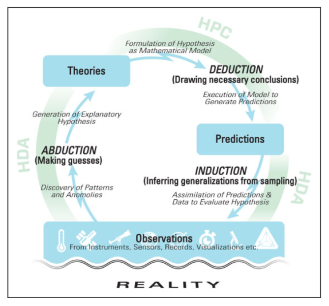
477 Asch, M. et al. (2018).
See also:
3.17 Implications for the realism debate
3.17.1 Introduction
See also:
3.17.2 Real clusters
- Nope: Hennig
See also:
3.17.3 Word meanings
- Inferential role semantics
- Wilfrid Sellars
- Word vectors
- Note that NLP has implications to the philosophy of language and realism
- Distributional semantics
- Olah, C. (2014). Deep learning, NLP, and representations.
- Kornai, A. (2023). Vector Semantics. 481
- NLP and Wittgenstein
- Perone, C.S. (2018). NLP word representations and the Wittgenstein philosophy of language. 482
- Belloni, M. (2019). Neural networks and philosophy of language: Why Wittgenstein’s theories are the basis of all modern NLP.
- Goldhill, O. (2019). Google Translate is a manifestation of Wittgenstein’s theory of language.
- Skelac, I. & Jandric, A. (2020). Meaning as use: From Wittgenstein to Google’s Word2vec. 483
- Theory of Vibe
- Grietzer, P. (2017). Ambient Meaning: Mood, Vibe, System. 484
- Grietzer, P. (2017). A theory of vibe. 485
- More discussion of NLP and meaning
- Tenney, I. et al. (2019). What do you learn from context? Probing for sentence structure in contextualized word representations. 486
- Nissim, M., van Noord, R., & van der Goot, R. (2019). Fair is better than sensational: Man is to doctor as woman is to doctor. 487
- Bender, E.M. & Koller, A. (2020). Climbing towards NLU: On meaning, form, and understanding in the age of data. 488
- Boccelli, D. (2022). Word embeddings align with Kandinsky’s theory of color.
- Elhage, N. et al. (2022). Toy models of superposition. 489
- Patel, R. & Pavlick, E. (2022). Mapping language models to grounded conceptual spaces. 490
- Lovering, C. & Pavlick, E. (2022). Unit testing for concepts in neural networks. 491
- Tweet by Joscha Bach, Mar 25, 2023
- Debate: Do language models need sensory grounding for meaning and understanding? (NYU).
- Piantadosi, S. (2023). Talk: Meaning in the age of large language models.
- Huh, M., Cheung, B., Wang, T., & Isola, P. (2024). The platonic representation hypothesis. 492
- Musser, G. (2024). Can an emerging field called neural systems understanding explain the brain.
- Jamali, M. et al. (2024). Semantic encoding during language comprehension at single-cell resolution. 493
- DisCoCat
- Categorical Compositional Distributional (DisCoCat) is a mathematical framework for natural language processing which uses category theory to unify distributional semantics with the principle of compositionality.
- Coecke, B., Sadrzadeh, M., & Clark, S. (2010). Mathematical foundations for a compositional distributional model of meaning. 494
- Grefenstette, E., Sadrzadeh, M. (2011). Experimental support for a categorical compositional distributional model of meaning. 495
- Balkir, E., Kartsaklis, D., & Sadrzadeh, M. (2015). Sentence entailment in compositional distributional semantics. 496
- Tyrrell, B. (2018). Applying distributional compositional categorical models of meaning to language translation. 497
- Kartsaklis, D. & Sadrzadeh, M. (2013). Prior disambiguation of word tensors for constructing sentence vectors. 498
- Grefenstette, E., Dinu, G., Zhang, Y.Z., Sadrzadeh, M., & Baroni, M. (2013). Multi-step regression learning for compositional distributional semantics. 499
- de Felice, G., Meichanetzidis, K., & Toumi, A. (2019). Functorial question answering. 500
481 Kornai (2023).
482 Perone (2018).
483 Skelac & Jandric (2020).
484 Grietzer (2017b).
485 Grietzer (2017a).
486 Tenney, I. et al. (2019).
487 Nissim, Noord, & Goot (2019).
488 Bender & Koller (2020).
489 Elhage, N. et al. (2022).
490 Patel & Pavlick (2022).
491 Lovering & Pavlick (2022).
492 Huh, Cheung, Wang, & Isola (2024).
493 Jamali, M. et al. (2024).
494 Coecke, Sadrzadeh, & Clark (2010).
495 Grefenstette & Sadrzadeh (2011).
496 Balkir, Kartsaklis, & Sadrzadeh (2015).
497 Tyrrell (2018).
498 Kartsaklis & Sadrzadeh (2013).
499 Grefenstette, E. et al. (2013).
500 de Felice, Meichanetzidis, & Toumi (2019).
Wittgenstein in PI:
and
One cannot guess how a word functions. One has to look at its use, and learn from that. 502
502 Wittgenstein (2009), §340.
Piantadosi:
Modern large language models integrate syntax and semantics in the underlying representations: encoding words as vectors in a high-dimensional space, without an effort to separate out e.g. part of speech categories from semantic representations, or even predict at any level of analysis other than the literal word. Part of making these models work well was in determining how to encode semantic properties into vectors, and in fact initializing word vectors via encodings of distribution semantics from e.g. Mikolov et al. 2013 (Radford et al. 2019). Thus, an assumption of the autonomy of syntax is not required to make models that predict syntactic material and may well hinder it. 503
503 Piantadosi (2023), p. 15.
See also:
3.18 My thoughts
My docs:
My talks:
3.19 Annotated bibliography
3.19.1 Mayo, D.G. (1996). Error and the Growth of Experimental Knowledge.
- Mayo (1996)
3.19.1.1 My thoughts
- TODO
3.19.2 Cowan, G. (1998). Statistical Data Analysis.
3.19.2.1 My thoughts
- TODO
3.19.3 James, F. (2006). Statistical Methods in Experimental Physics.
- F. James (2006)
3.19.3.1 My thoughts
- TODO
3.19.4 Cowan, G. et al. (2011). Asymptotic formulae for likelihood-based tests of new physics.
- Cowan et al. (2011)
- Glen Cowan, Kyle Cranmer, Eilam Gross, Ofer Vitells
3.19.4.1 My thoughts
- TODO
3.19.5 ATLAS Collaboration. (2012). Combined search for the Standard Model Higgs boson.
- ATLAS Collaboration (2012)
- arxiv:1207.0319
3.19.5.1 My thoughts
- TODO
3.19.6 Cranmer, K. (2015). Practical statistics for the LHC.
- Cranmer (2015)
3.19.6.1 My thoughts
- TODO
3.19.7 More articles to do
3.20 Links and encyclopedia articles
3.20.1 SEP
- Abduction
- Analysis of knowledge
- Bayes’ theorem
- Bayesian epistemology
- Carnap, Rudolf (1891-1970)
- Causal models
- Causal processes
- Confirmation
- Dutch book arguments
- Epistemology
- Foundationalist Theories of Epistemic Justification
- Hume, David (1711-1776)
- Identity of indiscernibles
- Induction, The problem of
- Logic and Probability
- Naturalized epistemology
- Peirce, Charles Sanders (1839-1914)
- Popper, Karl (1902-1994)
- Principle of sufficient reason
- Probability, Interpretations of
- Probabilistic pausation
- Reichenbach, Hans (1891-1953)
- Scientific explanation
- Scientific research and big data
- Statistics, Philosophy of
3.20.2 IEP
3.20.3 Scholarpedia
3.20.4 Wikipedia
- Abductive reasoning
- Akaike_information_criterion
- Algorithmic information theory
- Algorithmic probability
- Analysis of variance
- Aumann’s agreement theorem
- Bayes, Thomas (1701-1761)
- Bayesian inference
- Bernoulli, Jacob (1655-1705)
- Birnbaum, Allan (1923-1976)
- Bootstrapping
- Carnap, Rudolf (1891-1970)
- Confidence interval
- Cosmic variance
- Cramér-Rao bound
- Cramér, Harald (1893-1985)
- Data science
- Decision theory
- Deductive-nomological model
- Empiricism
- Epistemology
- Exploratory data analysis
- Fisher, Ronald (1890-1962)
- Frequentist inference
- Foundations of statistics
- Gauss, Carl Friedrich (1777-1855)
- German tank problem
- Gosset, William Sealy (1876-1937)
- Graunt, John (1620-1674)
- History of probability
- History of statistics
- Hume, David (1711-1776)
- Induction, The problem of
- Inductive reasoning
- Interval estimation
- Inverse probability
- Inverse problem
- Ivakhnenko, Alexey (1913-2007)
- Jeffrey, Richard (1926-2002)
- Jeffreys, Harold (1891-1989)
- Jeffreys prior
- Kolmogorov, Andrey (1903-1987)
- Kolmogorov complexity
- Lady tasting tea
- Laplace, Pierre-Simon (1749-1827)
- Likelihood principle
- Likelihoodist statistics
- List of important publications in statistics
- Machine learning
- Maximum likelihood estimation
- Mill, John Stuart (1806-1873)
- Misuse of p-values
- Neyman, Jerzy (1894-1981)
- Neyman construction
- Neyman-Pearson lemma
- Ockham, William of (1287-1347)
- Pearson, Egon (1895-1980)
- Pearson, Karl (1857-1936)
- Peirce, Charles Sanders (1839-1914)
- Poisson, Siméon Denis (1781-1840)
- Popper, Karl (1902-1994)
- Principle of sufficient reason
- Precision and recall
- Proteus phenomenon
- P-value
- Rao, C.R. (b. 1920)
- Replication crisis
- Rule of three
- Savage, Leonard Jimmie (1917-1971)
- Solomonoff, Ray (1926-2009)
- Solomonoff’s theory of inductive inference
- Statistical classification
- Statistical hypothesis testing
- Statistical inference
- Statistical sensitivity and specificity
- Statistical significance
- Statistics
- Statistics, Founders of
- Statistics, History of
- Statistics, Mathematical
- Statistics, Outline of
- Statistics, Philosophy of
- Student’s t-test
- Systematic error
- Thorp, Edward O. (b. 1932)
- Trial and error
- Tukey, John (1915-2000)
- Type-I and type-II errors
- Uncomfortable science
- Uniformitarianism
- Unsolved problems in statistics, List of
- Venn, John (1834-1923)
- Wilks, S.S. (1906-1964)
- Wilks’s theorem
3.20.5 Others
- Deep Learning: Our Miraculous Year 1990-1991 - Schmidhuber
- errorstatistics.com - Deborah Mayo’s blog
- Graunt, John (1620-1674) - statprob.com
- Peng, R. (2016). A Simple Explanation for the Replication Crisis in Science. - simplystatistics.org
- Why is binary classification not a hypothesis test? - stackexchange.com
- If the likelihood principle clashes with frequentist probability then do we discard one of them? - stackexchange.com
- Wilks’s theorem - fiveMinuteStats
- Dallal, G.E. (2012). The Little Handbook of Statistical Practice.
- Soch, J. et al. (2024). The Book of Statistical Proofs.