5 Covariance estimation
5.1 Introduction
This is where we discuss how to estimate \(\Sigma\).
- Estimation of covariance matrices
- Ayyala, D.N. (2020). High-dimensional statistical inference: Theoretical development to data analytics. 1
1 Ayyala (2020).
See my project:
Other software:
5.2 Sample mean and covariance
Mean:
\[ \mu_{i} = \mathbb{E}[x_{i}] \]
Covariance:
\[ \Sigma_{ij} = \mathrm{cov}(x_{i}, x_{j}) = \mathbb{E}[(x_{i} - \mu_{i})(x_{j} - \mu_{j})] = \mathbb{E}[x_{i} x_{j}] - \mu_{i} \mu_{j} \]
Sample mean:
\[ \bar{x}_{i} = \frac{1}{n} \sum_{k=1}^{n} x_{ik} \]
Sample covariance:
\[ V_{ij} = \frac{1}{n-1} \sum_{k=1}^{n} (x_{ik} - \bar{x}_{i}) ( x_{jk} - \bar{x}_{j} ) \]
Scatter matrix:
\[ S = \sum_{k=1}^{n} \left( \vec{x}_{k} - \vec{\mu} \right) \left( \vec{x}_{k} - \vec{\mu} \right)^\intercal \]
\[ V = \frac{1}{n-1} S \]
5.3 Online mean and covariance
This discusses how one can calculate a continuously updated covariance estimate one data sample at a time.
Univariate central moments:
\[ \mu_{p} = \mathbb{E}\left[(x - \mu_{1})^{p}\right] \]
\[ M_{p} = \sum_{i}^{n} (x_i - \mu_{1})^{p} \]
\[ \mu_{p} = \frac{M_{p}}{n} \,, \qquad \mu = \frac{M_{1}}{n} \,, \qquad \sigma^2 = \frac{M_{2}}{n} \]
Online mean:
\[ \delta \equiv x_n - \mu_{n - 1} \]
\[ \hat{\mu}_{n} = \mu_{n-1} + \frac{\delta}{n} \]
Online variance:
\[ S_{n} = M_{2,n} \]
\[ \hat{\sigma}^2 = \frac{S_{n}}{n-1} \]
where the \(n-1\) includes Bessel’s correction for sample variance.
Incrementally,
\[ S_{n} = S_{n-1} + (x_n - \mu_{n - 1}) (x_n - \mu_n) \]
Note that for \(n > 1\),
\[ (x_n - \mu_n) = \frac{n-1}{n} (x_n - \mu_{n - 1}) \]
Therefore,
\[ S_{n} = S_{n-1} + \frac{n-1}{n} (x_n - \mu_{n - 1}) (x_n - \mu_{n - 1}) \]
\[ S_{n} = S_{n-1} + \frac{n-1}{n} \delta^2 = S_{n-1} + \delta \left( \delta - \frac{\delta}{n} \right) \]
Online covariance (Welford algorithm):
\[ C_{n}(x, y) = C_{n-1} + (x_n - \bar{x}_{n - 1}) (y_n - \bar{y}_n) = C_{n-1} + \delta_{x} \delta_{y}^\prime \]
\[ C_{n}(x, y) = C_{n-1} + \frac{n-1}{n} (x_n - \bar{x}_{n - 1}) (y_n - \bar{y}_{n - 1}) = C_{n-1} + \frac{n-1}{n} \delta_{x} \delta_{y} \]
\[ \hat{V}_{xy} = \frac{C_{n}(x, y)}{n-1} \]
Matrix form:
\[ C_{n} = C_{n-1} + \left( \vec{x}_{n} - \vec{\mu}_{n-1} \right) \left( \vec{x}_{n} - \vec{\mu}_{n} \right)^\intercal = C_{n-1} + \vec{\delta} \: \vec{\delta^\prime}^\intercal \]
\[ C_{n} = C_{n-1} + \frac{n-1}{n} \left( \vec{x}_{n} - \vec{\mu}_{n-1} \right) \left( \vec{x}_{n} - \vec{\mu}_{n-1} \right)^\intercal = C_{n-1} + \frac{n-1}{n} S(\vec{x}_{n}, \vec{\mu}_{n-1}) \]
\[ \hat{V} = \frac{C_{n}}{n-1} \]
Note that the update term for the online covariance is a term in a scatter matrix, \(S\), using the currently observed data, \(\vec{x}_{n}\), and the previous means, \(\vec{\mu}_{n-1}\). But also note that the \(\vec{\delta} \: \vec{\delta^\prime}^\intercal\) form is also convenient because it comes naturally normalized and can be readily generalized for weighting.
Weighted mean:
\[ \hat{\mu}_{n} = \mu_{n-1} + \frac{w_{n,n}}{W_n} \delta = \mu_{n-1} + \frac{w_{n,n}}{W_n} (x_n - \mu_{n - 1}) \]
where
\[ W_{n} = \sum_{i=1}^{n} w_{n,i} \]
Weighted covariance:
\[ C_{n} = \frac{W_n - w_{n,n}}{W_{n-1}} C_{n-1} + w_{n,n} \left( x_{n} - \bar{x}_{n-1} \right) \left( y_{n} - \bar{y}_{n} \right) \]
\[ C_{n} = \frac{W_n - w_{n,n}}{W_{n-1}} C_{n-1} + w_{n,n} \left( \vec{x}_{n} - \vec{\mu}_{n-1} \right) \left( \vec{x}_{n} - \vec{\mu}_{n} \right)^\intercal \]
where
\[ \hat{V} = \frac{C_{n}}{W_{n}} \]
Exponential-weighted mean:
\[ \alpha = 1 - \mathrm{exp}\left( \frac{-\Delta{}t}{\tau} \right) \simeq \frac{\Delta{}t}{\tau} \]
\[ \hat{\mu}_{n} = \mu_{n-1} + \alpha (x_{n} - \mu_{n-1}) = (1 - \alpha) \mu_{n-1} + \alpha x_{n} \]
Exponential-weighted covariance:
\[ C_{n} = (1 - \alpha) C_{n-1} + \alpha \left( x_{n} - \bar{x}_{n-1} \right) \left( y_{n} - \bar{y}_{n} \right) \]
\[ C_{n} = (1 - \alpha) C_{n-1} + \alpha \left( \vec{x}_{n} - \vec{\mu}_{n-1} \right) \left( \vec{x}_{n} - \vec{\mu}_{n} \right)^\intercal \]
where by summing a geometric series, one can show that for exponential weighting, \(W_{n} = 1\), so \(\hat{V} = C_{n}\).
See:
- Algorithms for calculating variance
- Welford, B.P. (1962). Note on a method for calculating corrected sums of squares and products. 2
- Neely, P.M. (1966). Comparison of several algorithms for computation of means, standard deviations and correlation coefficients. 3
- Youngs, E.A. & Cramer, E.M. (1971). Some results relevant to choice of sum and sum-of-product algorithms. 4
- Ling, R.F. (1974). Comparison of several algorithms for computing sample means and variances. 5
- Chan, T.F., Golub, G.H., & LeVeque, R.J. (1979). Updating formulae and a pairwise algorithm for computing sample variances. 6
- Pébay, P. (2008). Formulas for robust, one-pass parallel computation of covariances and arbitrary-order statistical moments. 7
- Finch, T. (2009). Incremental calculation of weighted mean and variance. 8
- Cook, J.D. (2014). Accurately computing running variance.
- Meng, X. (2015). Simpler online updates for arbitrary-order central moments. 9
- Pébay, P., Terriberry, T.B., Kolla, H. & Bennett, J. (2016). Numerically stable, scalable formulas for parallel and online computation of higher-order multivariate central moments with arbitrary weights. 10
- Schubert, E. & Gertz, M. (2018). Numerically stable parallel computation of (co-)variance. 11
- Chen, C. (2019). Welford algorithm for updating variance.
5.4 Variance-correlation decomposition
Covariance:
\[ \Sigma_{ij} = \mathrm{cov}(x_{i}, x_{j}) = \mathbb{E}[(x_{i} - \mu_{i})(x_{j} - \mu_{j})] = \mathbb{E}[x_{i} x_{j}] - \mu_{i} \mu_{j} \]
Standard deviation:
\[ \sigma_{i} = \sqrt{\Sigma_{ii}} \]
Correlation:
\[ R_{ij} = \frac{\Sigma_{ij}}{\sqrt{\Sigma_{ii}\Sigma_{jj}}} = \frac{\Sigma_{ij}}{\sigma_{i}\sigma_{j}} \]
Beta:
\[ \beta_{i} = \frac{\mathrm{cov}(x_{i}, x_{m})}{\mathrm{var}(x_{m})} = \frac{\Sigma_{im}}{\Sigma_{mm}} = R_{im} \frac{\sigma_{i}}{\sigma_{m}} \]
Variance-correlation decomposition:
\[ \Sigma = D R D \]
where
\[ D = \mathrm{diag}(\sigma_{1}, \ldots, \sigma_{n}) \]
5.5 Precision-partial-correlation decomposition
Precision:
\[ \Omega = \Sigma^{-1} \]
We will derive something similar to the variance-correlation decomposition, \(\Sigma = D R D\), except for precision. To motivate its form, it helps to know that a conditional covariance matrix is the inverse of a diagonal partition of a precision matrix.
Schur complement lemma (TODO: prove or motivate): 12
12 Bishop (2024), p. 76–81. TODO: Need to clarify which details rely on the data being Gaussian. Claude warns:
For any multivariate distribution with finite second moments: \(\mathrm{cov}(x_{1}|x_{2}) = \Sigma_{11} - \Sigma_{12}\Sigma_{22}^{-1}\Sigma_{21}\)
But this only equals \(\Omega_{11}^{-1}\) under Gaussianity. See also Styan (1983).
\[ \Sigma_{A|B} = \Omega_{AA}^{-1} = \Sigma_{AA} - \Sigma_{AB} \Sigma_{BB}^{-1} \Sigma_{BA} \]
First, let us consider a partition where \(A\) is only one variable and \(B\) has the rest.
\[ A = \{ x_{i} \} \qquad B = \{ \mathrm{rest} \} \]
In this case, \(\Omega_{AA}^{-1} = \Omega_{ii}^{-1}\) shows that the diagonal elements of the precision, \(\Omega_{ii}\), are related to partial variances given by
\[ \tau_{i}^{2} = \left[\Sigma_{A|B}\right]_{ii} = \Omega_{ii}^{-1} = \frac{1}{\Omega_{ii}} \]
since \(\Omega_{ii}\) is a scalar.
Now let us partition our observable variables into two sets:
\[ A = \{ x_{i}, x_{j} \} \qquad B = \{ \mathrm{rest} \} \]
The conditional covariance is equivalent to the covariance of the residuals when fitting the rest of the variables (TODO: motivate).
\[ \Sigma_{ij|\mathrm{rest}} = \mathrm{cov}(x_{i}, x_{j} | \mathrm{rest}) = \mathrm{cov}(\varepsilon_{i}, \varepsilon_{j}) \]
Again, looking at \(\Omega_{AA}^{-1}\), we have
\[ \Sigma_{A|B} = \Omega_{AA}^{-1} = \begin{pmatrix} \Omega_{ii} & \Omega_{ij} \\ \Omega_{ji} & \Omega_{jj} \end{pmatrix}^{-1} = \frac{1}{\Delta} \begin{pmatrix} \Omega_{jj} & - \Omega_{ij} \\ - \Omega_{ji} & \Omega_{ii} \end{pmatrix} \]
where \(\Delta \equiv \mathrm{det} \Omega_{AA}\). From this we note that the off-diagonal elements of \(\Omega_{ij}\) are proportional to the negative conditional covariance.
Similar to the definition of correlation, \(R_{ij}\), we define the (off-diagonal) partial correlation as
\[ P_{ij} = \frac{\left[\Sigma_{A|B}\right]_{ij}}{\sqrt{\left[\Sigma_{A|B}\right]_{ii}\left[\Sigma_{A|B}\right]_{jj}}} = \frac{-\frac{1}{\Delta}\Omega_{ij}}{\sqrt{\frac{1}{\Delta}\Omega_{jj}\frac{1}{\Delta}\Omega_{ii}}} = \frac{-\Omega_{ij}}{\sqrt{\Omega_{ii}\Omega_{jj}}} = - \tau_{i} \Omega_{ij} \tau_{j} \]
and equivalently
\[ P_{ij} = \mathrm{corr}(x_{i}, x_{j} | \mathrm{rest}) = \mathrm{corr}(\varepsilon_{i}, \varepsilon_{j}) \]
Importantly, \(x_i\) and \(x_j\) are conditionally independent iff \(P_{ij} = 0\).
TODO: Expand on why precision matrices are often naturally sparse as related to Gaussian Graphical Models. See discussion in Chan & Kroese. 13
13 J. C. C. Chan & Kroese (2025), p. 371–2.
We have that the elements of the precision are
\[ \Omega_{ii} = \frac{1}{\tau_{i}^{2}} \qquad \Omega_{ij} = - \frac{1}{\tau_{i}} P_{ij} \frac{1}{\tau_{j}} \]
Combining our results shows that precision can be factored as
\[ \Omega = \begin{pmatrix} \frac{1}{\tau_1} & 0 & 0 & \cdots & 0 \\ 0 & \frac{1}{\tau_2} & 0 & \cdots & 0 \\ 0 & 0 & \frac{1}{\tau_3} & \cdots & 0 \\ \vdots & \vdots & \vdots & \ddots & \vdots \\ 0 & 0 & 0 & \cdots & \frac{1}{\tau_n} \end{pmatrix} \begin{pmatrix} 1 & - P_{12} & - P_{13} & \cdots & - P_{1n}\\ - P_{21} & 1 & - P_{23} & \cdots & - P_{2n} \\ - P_{31} & - P_{32} & 1 & \cdots & - P_{3n} \\ \vdots & \vdots & \vdots & \ddots & \vdots \\ - P_{n1} & - P_{n2} & - P_{n3} & \cdots & 1 \end{pmatrix} \begin{pmatrix} \frac{1}{\tau_1} & 0 & 0 & \cdots & 0 \\ 0 & \frac{1}{\tau_2} & 0 & \cdots & 0 \\ 0 & 0 & \frac{1}{\tau_3} & \cdots & 0 \\ \vdots & \vdots & \vdots & \ddots & \vdots \\ 0 & 0 & 0 & \cdots & \frac{1}{\tau_n} \end{pmatrix} \]
In order to factor-out a minus sign and consistently get the diagonal elements \(\Omega_{ii}\) to come out positive and have \(P_{ii} = 1\), we can define the partial correlation matrix as 14
14 This form is nicely clarified in Erickson & Rydén (2025). If one does not add \(2I\), then you have to use a convention where \(P_{ii} = -1\). In either convention, the off-diagonals are what is meaningful, and \(P_{ij} > 0\) indicates a positive partial correlation.
\[ P = - T \: \Omega \: T + 2 I \]
where
\[ T = \mathrm{diag}(\tau_{1}, \ldots, \tau_{n}) \]
and
\[ \tau_{i} = \frac{1}{\sqrt{\Omega_{ii}}} \]
are the partial standard deviations.
So equivalently, the precision-partial-correlation decomposition is
\[ \Omega = T^{-1} (-P + 2I) T^{-1} \]
See:
- Covariance matrix
- Partial correlation
- Marsaglia, G. (1964). Conditional means and covariances of normal variables with singular covariance matrix. 15
- Dempster, A.P. (1972). Covariance selection. 16
- Knuiman, M. (1978). Covariance selection. 17
- Whittaker, J. (1990). Graphical Models in Applied Multivariate Statistics. 18
- Edwards, D. (1995). Introduction to Graphical Modelling. 19
- Lauritzen, S. (1996). Graphical Models. 20
- Wong, F., Carter, C. K., & Kohn, R. (2003). Efficient estimation of covariance selection models. 21
- Zhang, F. (2005). The Schur Complement and its Applications. 22
- Bolla, M. (2023). Partitioned covariance matrices and partial correlations. 23
15 Marsaglia (1964).
16 Dempster (1972).
17 Knuiman (1978).
18 Whittaker (1990).
19 Edwards (1995).
20 Lauritzen (1996).
21 Wong, Carter, & Kohn (2003).
22 Zhang (2005).
23 Bolla (2023).
Timeline of graphical models by Claude:
- 1972: Dempster establishes covariance selection and precision matrix sparsity
- 1990: Whittaker provides comprehensive GGM textbook treatment
- 1995: Edwards expands the graphical modeling framework
- 1996: Lauritzen gives rigorous mathematical foundations including partial correlation formulas
- 2003: Wong et al. formalize the precision matrix factorization
- 2007+: Modern computational methods (graphical lasso, etc.) build on these foundations
More:
- Galloway, M. (2019). Shrinking characteristics of precision matrix estimators: An illustration via regression. 24
- Bax, K., Taufer, E., & Paterlini, S. (2022). A generalized precision matrix for t-Student distributions in portfolio optimization. 25
- Dutta, S. & Jain, S. (2023). Precision versus shrinkage: A comparative analysis of covariance estimation methods for portfolio allocation. 26
5.6 Shrinkage estimators
- Shrinkage
- Ledoit, O. & Wolf, M. (2001). Honey, I shrunk the sample covariance matrix. 27
- Ledoit, O. & Wolf, M. (2003). Improved estimation of the covariance matrix of stock returns with an application to portfolio selection. 28
- Coqueret, G. & Milhau, V. (2014). Estimating covariance matrices for portfolio optimization 29
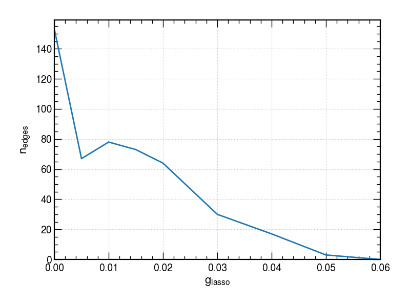
5.7 Graphical lasso
Graphical lasso:
\[ \hat{\Omega} = \underset{\Omega}{\mathrm{argmin}} \: \left( \mathrm{tr}(S \Omega) - \mathrm{log}(\mathrm{det}(\Omega)) + g \left\lVert \Omega \right\lVert_\mathrm{1} \right) \]
where \(\left\lVert \Omega \right\lVert_\mathrm{1}\) is the sum of the absolute values of off-diagonal elements of \(\Omega\).
See:
- Graphical lasso
- Graphical lasso in the scikit-learn user guide
- Banerjee, O., d’Aspremont, A., & Ghaoui, L.E. (2005). Sparse covariance selection via robust maximum likelihood estimation. 30
- Friedman, J., Hastie, T. and Tibshirani, R. (2008). Sparse inverse covariance estimation with the graphical lasso. 31
- Mazumder, R. & Hastie, T. (2011). The graphical lasso: New insights and alternatives. 32
- Chang, B. (2015). An introduction to graphical lasso. 33
- Fan, J., Liao, Y., & Liu, H. (2015). An overview on the estimation of large covariance and precision matrices. 34
- Maxime, A. (2015). Inverse covariance matrix regularization for minimum variance portfolio. 35
- Erickson, S. & Rydén, T. (2025). Inverse covariance and partial correlation matrix estimation via joint partial regression. 36
5.8 Eigendecomposition
Eigendecomposition of \(\Sigma\):
\[ \Sigma = Q \: \Lambda \: Q^{-1} \]
where
\[ \Lambda = \mathrm{diag}(\lambda_{1}, \ldots, \lambda_{n}) \]
contains the eigenvalues of \(\Sigma\) and
\[ Q = \mathrm{cols}(\vec{q}_{1}, \ldots, \vec{q}_{n}) \]
contains the eigenvectors. Note that since \(\Sigma\) is symmetric that guarantees that \(Q\) is orthogonal, \(Q^{-1} = Q^{\intercal}\).
For any analytic function, \(f\),
\[ f(\Sigma) = Q \: f(\Lambda) \: Q^{-1} = Q \: \mathrm{diag}(f(\lambda)) \: Q^{-1} \]
Sqrt covariance matrix:
\[ \sqrt{\Sigma} = Q \: \sqrt{\Lambda} \: Q^{-1} = Q \: \mathrm{diag}(\sqrt{\lambda}) \: Q^{-1} \]
See:
- Open Source Quant: Square root of a portfolio covariance matrix
- Principal component analysis (PCA)
- Deng, W., Polak, P., Safikhani, A., & Shah, R. (2024). A unified framework for fast large-scale portfolio optimization. 37
37 Deng, Polak, Safikhani, & Shah (2024).
5.9 Geometry of covariance
- Rousseeuw, P.J. & Molenberghs, G. (1994). The shape of correlation matrices. 38
38 Rousseeuw & Molenberghs (1994).