4 Portfolio theory
4.1 Introduction
Given some menu of possible investments, what mix should we hold? How should we hold value through time?
Mean-variance analysis is part of fundamental analysis, specifically within modern portfolio theory (MPT). Developed by Harry Markowitz in 1952 and later expanded by William Sharpe, it focuses on analyzing fundamental characteristics of securities, specifically their expected returns (mean) and risk (variance), to construct optimal portfolios.
4.2 Modern portfolio theory
4.2.1 History and pedagogy
Keywords:
- Modern portfolio theory (MPT)
- Harry Markowitz (1927-2023)
- Markowitz model
- Sharpe ratio
Historical background:
- Markowitz, H.M. (1952). Portfolio selection. 1
- Roy, A.D. (1952). Safety first and the holding of assets. 2
- Markowitz, H.M. (1959). Portfolio Selection: Efficient Diversification of Investments. 3
- Merton, R.C. (1972). An analytic derivation of the efficient portfolio frontier. 4
- Levy, H. & Markowitz, H.M. (1979). Approximating expected utility by a function of mean and variance. 5
- In 1990, Harry Markowitz, Merton Miller, and William F. Sharpe were awarded the Nobel Prize in Economics “for their pioneering work in the theory of financial economics”.
- Markowitz, H.M. (1990). Nobel lecture: Foundations of portfolio theory. 6
- Markowitz, H.M. (2005). Market efficiency: A theoretical distinction and so what? 7
1 Markowitz (1952).
2 Roy (1952).
3 Markowitz (1959).
4 Merton (1972).
5 Levy & Markowitz (1979).
6 Markowitz (1990).
7 Markowitz (2005).
Pedagogy:
- Luenberger, D.G. (1998). Investment Science. 8
- Palomar, D.P. (2025). Portfolio Optimization: Theory and Application. 9
Lecture notes:
- Armerin, F. (2023). Lecture notes: More on mean-variance analysis.
- Caflisch, R. (2003). Lecture notes: Mathematics of Finance.
- Das, S.R. (2016). Data Science: Theories, Models, Algorithms, and Analytics. 10
- Also: Das, S.R. (2017). Being mean with variance: Markowitz optimization.
- Ireland, P. (2013). Lecture notes: Principles of Macroeconomics.
- Ireland, P. (2024). Lecture notes: Mathematics for Economists.
- Ireland, P. (2025). Lecture notes: Financial Economics.
- In particular, Lecture 6
- Kasa, K. (2023). Lecture notes by Ken Kasa (SFU)
- In particular, Lecture 7
- Kwok, Y.K. (2017). Lecture notes: Fundamentals of Mathematical Finance. 11
- In particular, Lecture 2
- Sigman, K. (2005). Notes on fund theorems.
- Tam, A.S. (2021). Lagrangians and portfolio optimization.
4.2.2 Markowitz portfolio problem
Given an expected covariance, \(V\), and expected returns, \(\vec{\mu}\), we want to find the portfolio with the best return per risk. How to estimate \(V\) will be discussed in more detail in Chapter 5.
Return of a portfolio:
\[ r = \vec{w}^\intercal \, \vec{\mu} = \sum_i w_{i} \, \mu_{i} \]
Variance of a portfolio:
\[ \sigma^2 = \vec{w}^\intercal \, V \, \vec{w} = \sum_{ij} w_{i} \, V_{ij} \, w_{j} \]
TODO: Show above 12
12 Luenberger (1998), p. 150.
Given an \(n\)-dimensional vector of expected returns, \(\vec{\mu}\), an \(n\times{}n\)-dimensional expected covariance matrix, \(V\), an \(m\times{}n\)-dimensional constraint matrix, \(A\), an \(m\)-dimensional constraint vector, \(\vec{b}\), and a target return, \(r_{\ast}\), solve for the portfolio weights, \(\vec{w}_{\ast}\), an \(n\)-dimensional vector, that are efficient, i.e. those that minimize the standard deviation of the portfolio return, \(\sigma\), for a given target return. Return \((\vec{w}_{\ast}, \sigma_{\ast})\). 13
Solve
\[ \vec{w}_{\ast} = \underset{w}{\mathrm{argmin}}\ \vec{w}^\intercal \, V \, \vec{w} \]
such that
\[ \vec{w} \cdot \vec{1} = 1 \]
\[ \vec{w} \cdot \vec{\mu} = r_{\ast} \]
and with further optional constraints
\[ A \, \vec{w} \geq \vec{b} \]
13 Markowitz (1959), p. 172.
There are a lot of topics to discuss about solving for the efficient frontier:
- How there is an analytic solution if you allow shorts
- Solving with Lagrange multipliers
- Solving with numerical convex optimization
TODO: Discuss the above more.
It can be shown14 that there is an analytic solution where:
14 Merton (1972) was the first to show there was an analytic solution to the Markowitz portfolio problem? For the analytic results descussed here, we generally follow Kwok (2017). Note that we use variable names following Kwok, whereas to convert from Merton to Kwok: \(a_\mathrm{M} = b_\mathrm{K}\), \(b_\mathrm{M} = c_\mathrm{K}\), \(c_\mathrm{M} = a_\mathrm{K}\).
\[ a \equiv \vec{1}^\intercal \, V^{-1} \, \vec{1}, \qquad b \equiv \vec{1}^\intercal \, V^{-1} \, \vec{\mu}, \qquad c \equiv \vec{\mu}^\intercal \, V^{-1} \, \vec{\mu}, \qquad d \equiv a\,c - b^2 \]
There are two efficient portfolios of note: the minimum variance portfolio, \(\vec{w}_\mathrm{min}\), and the tangent portfolio, \(\vec{w}_\mathrm{tan}\).
The minimum variance portfolio is
\[ \vec{w}_\mathrm{min} = \frac{V^{-1} \, \vec{1}}{a} = \frac{V^{-1} \, \vec{1}}{\vec{1}^\intercal \, V^{-1} \, \vec{1}} \]
It has a return
\[ r_\mathrm{min} = \vec{w}_\mathrm{min} \cdot \vec{\mu} = \frac{\vec{1}^\intercal \, V^{-1} \, \vec{\mu}}{a} = \frac{b}{a} \]
and a variance
\[ \sigma_\mathrm{min}^2 = \vec{w}_\mathrm{min}^\intercal \, V \, \vec{w}_\mathrm{min} = \left( \frac{\vec{1}^\intercal \, V^{-1}}{a} \right) V \left( \frac{V^{-1} \, \vec{1}}{a} \right) = \frac{\vec{1}^\intercal \, V^{-1} \, \vec{1}}{a^2} = \frac{1}{a} \]
The tangent portfolio is
\[ \vec{w}_\mathrm{tan} = \frac{V^{-1} \, \vec{\mu}}{b} = \frac{V^{-1} \, \vec{\mu}}{\vec{1}^\intercal \, V^{-1} \, \vec{\mu}} \]
It has a return
\[ r_\mathrm{tan} = \vec{w}_\mathrm{tan} \cdot \vec{\mu} = \frac{\vec{\mu}^\intercal \, V^{-1} \, \vec{\mu}}{b} = \frac{c}{b} \]
and a variance
\[ \sigma_\mathrm{tan}^2 = \vec{w}_\mathrm{tan}^\intercal \, V \, \vec{w}_\mathrm{tan} = \left( \frac{\vec{\mu}^\intercal \, V^{-1}}{b} \right) V \left( \frac{V^{-1} \, \vec{\mu}}{b} \right) = \frac{\vec{\mu}^\intercal \, V^{-1} \, \vec{\mu}}{b^2} = \frac{c}{b^2} \]
The efficient frontier can be written as a linear combination of any two efficient portfolios. This is discussed in more detail in the section on Fund theorems. Written as a combination of the minimum variance and the tangent portfolios gives
\[ \vec{w}_{\ast} = \psi \, \vec{w}_\mathrm{min} + (1-\psi) \, \vec{w}_\mathrm{tan} \]
where
\[ \psi = (c - b \, r_{\ast}) \, a \, / \, d \]
The efficient frontier portfolio can be equivalently written
\[\begin{align} \vec{w}_{\ast} &= \psi \, \vec{w}_\mathrm{min} + (1-\psi) \, \vec{w}_\mathrm{tan} \\ &= \left( \frac{c - b \, r_{\ast}}{d} \right) a \, \vec{w}_\mathrm{min} + \left( \frac{a \, r_{\ast} - b}{d} \right) b \, \vec{w}_\mathrm{tan} \\ &= \left( \frac{c - b \, r_{\ast}}{d} \right) V^{-1} \, \vec{1} + \left( \frac{a \, r_{\ast} - b}{d} \right) V^{-1} \, \vec{\mu} \end{align}\]
Along the frontier, the return is
\[ r_{\ast} = \psi \, r_\mathrm{min} + (1-\psi) \, r_\mathrm{tan} \]
The variance is
\[ \sigma^2_{\ast} = \frac{a}{d} \, r_{\ast}^{2} - \frac{2 \, b}{d} \, r_{\ast} + \frac{c}{d} \]
TODO: Note calculation order of \(\vec{w}_\mathrm{min}(\mu, V)\) and \(\vec{w}_\mathrm{tan}(\mu, V, r_\mathrm{f})\), then calculate \(r_{\ast}(\sigma_{\ast})\), scanning from \(\sigma_\mathrm{min}\) to \(\sigma_\mathrm{max}\).
In general, depending on the correlations of the assets, the efficient frontier portfolios will short various positions, indicated by having negative weights.
4.2.3 No-shorts frontier
If one adds an additional constraint to the Markowitz portfolio problem as stated, requiring that we don’t short any positions
\[ w_i \geq 0 \]
then the problem doesn’t have an analytic solution. TODO: Citation needed.
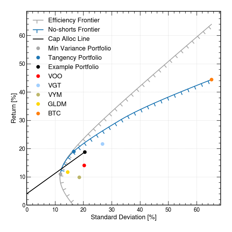
The no-shorts frontier can be solved numerically with quadratic programming. In general, the no-shorts frontier will follow the unconstrained efficient frontier when there isn’t any shorting in the efficient portfolios, and the no-shorts frontier will pull away from the efficient frontier to somewhat lower returns when there is shorting on the efficient frontier.
An example of the efficient frontier and the no-shorts frontier is shown in Figure 4.2.
Quadratic programming and convex optimization are discussed in more detail in Chapter 6.
4.2.4 Efficient-market hypothesis
- Efficient-market hypothesis
- Eugene Fama (b. 1939)
- Fama, E.F. (1965). The behavior of stock-market prices. 15
- Fama, E.F. (1970). Efficient capital markets: A review of theory and empirical work. 16
See also:
4.2.5 Lessons of MPT
Markowitz:
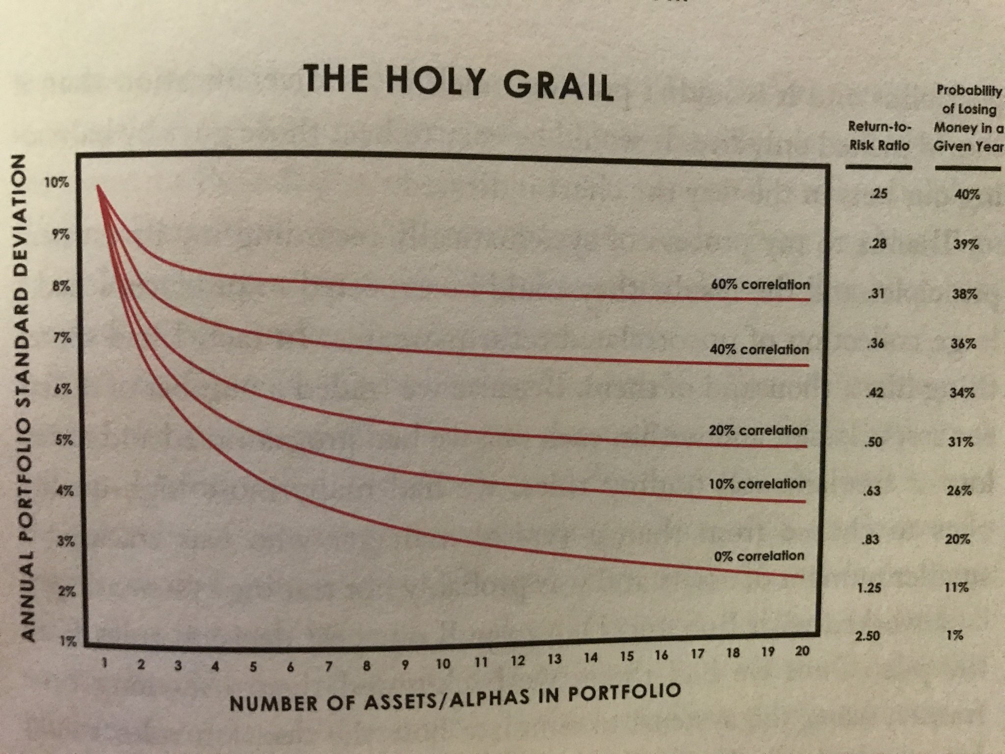
[I]n trying to make variance small it is not enough to invest in many securities. It is necessary to avoid investing in securities with high covariances among themselves. We should diversify across industries because firms in different industries, especially industries with different economic characteristics, have lower covariances than firms within an industry. 17
17 Markowitz (1952), p. 89.
Dalio: “The Holy Grail of investing”, see Figure 4.3.
Inverse variance portfolio
Let us look at the minimum variance portfolio, which does not depend on estimating the returns.
\[ \vec{w}_\mathrm{min} = \frac{V^{-1} \, \vec{1}}{a} = \frac{V^{-1} \, \vec{1}}{\vec{1}^\intercal \, V^{-1} \, \vec{1}} \]
Consider the simplest and favorable case that the assets are uncorrelated, \(V_{ij} = 0\), for \(i \neq j\), and then \(V_{ii}^{-1} = \frac{1}{V_{ii}} = \frac{1}{\sigma_{i}^{2}}\).
Therefore the minimum variance portfolio for uncorrelated assets is the inverse variance portfolio (IVP):
\[ \left[ \vec{w}_\mathrm{IVP} \right]_{i} = \eta \, \frac{1}{\sigma_{i}^{2}} \]
where \(\eta\) is a normalization constant, \(\eta = \left( \sum_{i} \frac{1}{\sigma_{i}^{2}} \right)^{-1}\).
4.3 Fund theorems
4.3.1 Mutual fund separation theorem
- Mutual fund separation theorem
- Cass, D. & Stiglitz, J.E. (1970). The structure of investor preferences and asset returns, and separability in portfolio allocation: A contribution to the pure theory of mutual funds. 18
- Chamberlain, G. (1983). A characterization of the distributions that imply mean-variance utility functions. 19
- Owen, J. & Rabinovitch, R. (1983). On the class of elliptical distributions and their applications to the theory of portfolio choice. 20
Cass & Stiglitz:
[G]iven a market in which there are available \(n\) different assets, nonetheless all the opportunities relevant to the investor’s decision can be provided by a set of \(m\) (\(< n\)) “mutual funds,” i.e., a set of \(m\) linear combinations (with weights adding to one) of the available assets. 21
21 Cass & Stiglitz (1970), p. 122.
4.3.2 Two-fund theorem
Continuing the discussion of the context of a portfolio of risky assets (no risk-free asset; to be considered in the next section).
Tobin22 is often credited as the first to note, and later Merton23 exposited more formally, the Two-fund theorem:
Merton:
Given \(m\) assets satisfying the conditions […], there are two portfolios (“mutual funds”) constructed from these \(m\) assets, such that all risk-averse individuals, who choose their portfolios so as to maximize utility functions dependent only on the mean and variance of their portfolios, will be indifferent in choosing between portfolios from among the original \(m\) assets or from these two funds. 24
24 Merton (1972), p. 1858.
Kasa:
Any portfolio on the efficient frontier can be written as a linear combination of two fixed efficient portfolios.
\[ \vec{w}_{\ast} = \psi \, \vec{w}_{1} + (1-\psi) \, \vec{w}_{2} \]
TODO: reparameterize? 25
25 TODO: Throughout this we have parameterized \(\psi\) such as it goes from 0 to 1, we go from holding asset 2 to 1. Let’s reparameterize so that \(\psi \rightarrow (1-\psi)\).
4.3.3 One-fund theorem
Now we consider adding the posibility of holding a risk-free asset with a risk-free return, \(r_\mathrm{f}\).
One-fund theorem:
Kwok:
Any efficient portfolio can be expressed as a [linear] combination of the risk free asset and the portfolio (or fund) represented by \(M\).
Kasa:
Any portfolio on the efficient frontier can be written as a linear combination of one fixed efficient non-risk-free portfolio and the risk-free asset.
The portfolio weights are
\[ \vec{w}_{\ast} = \kappa \, \vec{w}_\mathrm{f} + (1-\kappa) \, \vec{w}_\mathrm{tan} \]
The portfolio return is
\[ r_{\ast} = \kappa \, r_\mathrm{f} + (1-\kappa) \, r_\mathrm{tan} \]
The portfolio standard deviation is
\[ \sigma_{\ast} = \left| 1-\kappa \right| \sigma_\mathrm{tan} \]
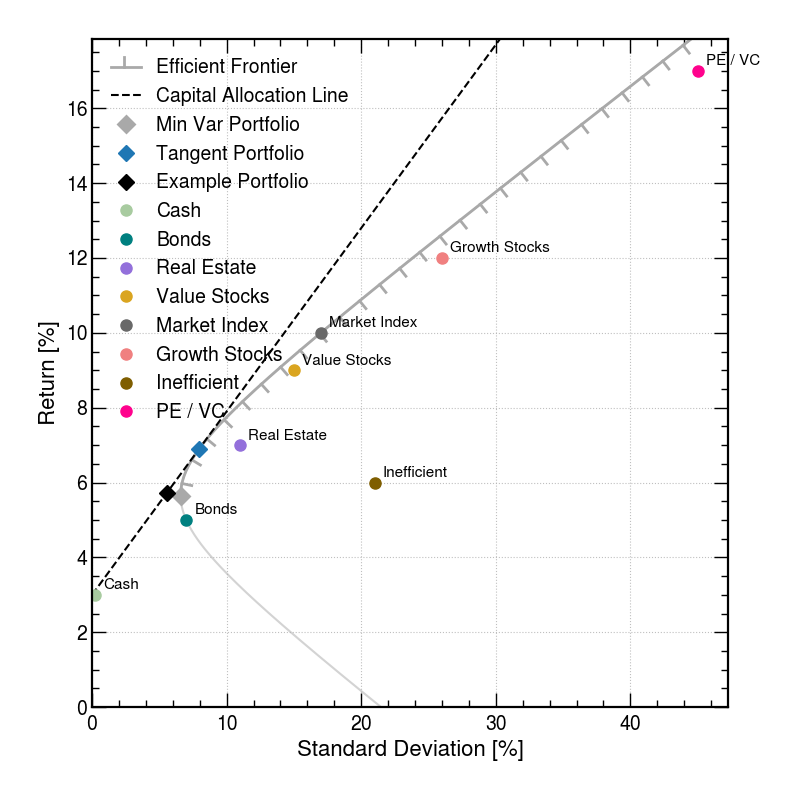
Since the efficient frontier is a linear combination of the risk-free, “cash”, and a single portfolio of risky assets, “stocks”, then it forms a line in return-risk-space from the risk-free asset to the tangent portfolio, and follows the line further up if one allows borrowing at the risk-free rate and investing in the tangent portfolio. This line is called the Capital Allocation Line because it represents the possible portfolios one can have depending on how much of their cash they have deployed into risky assets in the market.
The functional form of the Capital Allocation Line is
\[ r_\mathrm{CAL}(\sigma) = r_\mathrm{f} + \sigma \, \sqrt{ a \, r_\mathrm{f}^{2} - 2 \, b \, r_\mathrm{f} + c} \]
TODO: Double-check the expression and example values of this slope.
Note that while the shape of the efficient frontier is unchanged by introducing or varying the risk-free rate of return, which portfolio along the frontier that is the tangent portfolio will depend on the risk-free rate of return.
The tangent portfolio with a risk-free asset is
\[ \vec{w}_\mathrm{tan} = \frac{V^{-1} \, (\vec{\mu} - r_\mathrm{f} \, \vec{1})}{\vec{1}^\intercal \, V^{-1} \, (\vec{\mu} - r_\mathrm{f} \, \vec{1})} \]
It has a return
\[ r_\mathrm{tan} = \vec{\mu} \cdot \vec{w}_\mathrm{tan} = \frac{c - b \, r_\mathrm{f}}{b - a \, r_\mathrm{f}} \]
and a variance
\[ \sigma_\mathrm{tan}^{2} = \frac{\left|\vec{\mu} - r_\mathrm{f} \, \vec{1}\right|^2}{ (\vec{\mu} - r_\mathrm{f} \, \vec{1})^\intercal \, V^{-1} \, (\vec{\mu} - r_\mathrm{f} \, \vec{1})} = \frac{a \, r_\mathrm{f}^2 - 2 \, b \, r_\mathrm{f} + c}{(b - a \, r_\mathrm{f})^2} \]
The tangent portfolio is the portfolio with the maximum Sharpe ratio, \(S_i\).
\[ S_i \equiv \frac{ r_i - r_\mathrm{f} }{ \sigma_i } \]
The Sharpe ratio is a measure of how much excess return an asset had over a risk-free asset, adjusted for the risk as measured by the standard deviation of return.
TODO:
- Citation needed for the one-fund theorem
- Related to the efficient-market hypothesis: in equilibrium, the tangent portfolio becomes the market portfolio
4.4 Capital asset pricing model
Keywords:
- Capital Asset Pricing Model (CAPM)
- William F. Sharpe (b. 1934)
- Beta
- Alpha
- Security Characteristic Line (SCL)
- Security Market Line (SML)
- Jensen’s alpha
- Treynor ratio
Background:
- Sharpe, W.F. (1963). A simplified model for portfolio analysis. 26
- Sharpe, W.F. (1964). Capital asset prices: A theory of market equilibrium under conditions of risk. 27
- Lintner, J. (1965). The valuation of risk assets and the selection of risky investments in stock portfolios and capital budgets. 28
- Fama, E.F. (1968). Risk, return and equilibrium: Some clarifying comments. 29
- Jensen, M. (1968). The performance of mutual funds in the period 1945-1964. 30
- Sharpe, W.F. (1990). Nobel lecture: Capital asset prices with and without negative holdings. 31
- Sharpe, W.F. (1999). Portfolio Theory and Capital Markets. 32
- Fama, E.F. & French, K.R. (2004). The capital ssset pricing model: Theory and evidence. 33
- Kolari, J.W. & Pynnönen, S. (2023). Investment Valuation and Asset Pricing. 34
26 Sharpe (1963).
27 Sharpe (1964).
28 Lintner (1965).
29 Fama (1968).
30 Jensen (1968).
31 Sharpe (1990).
32 Sharpe (1999).
33 Fama & French (2004).
34 Kolari & Pynnönen (2023).
The CAPM model return is
\[ r_\mathrm{CAPM} = r_\mathrm{f} + \alpha_i + \beta_i \, (r_\mathrm{m} - r_\mathrm{f}) \]
Thought in \(r - r_\mathrm{f}\) vs \(r_\mathrm{m} - r_\mathrm{f}\) space, accumulating points over time, \(\alpha_{i}\) and \(\beta_{i}\) can be calculated via linear regression, minimizing the Sum Squared Errors:
\[ \mathrm{SSE} = \sum_{t=1}^{T} \varepsilon_{it} = \sum_{t=1}^{T} \left( r_{it} - r_{\mathrm{CAPM}t} \right)^2 = \sum_{t=1}^{T} \left( r_{it} - r_{\mathrm{f}t} - \alpha_i - \beta_i \, (r_{\mathrm{m}t} - r_{\mathrm{f}t}) \right)^2 \]
Let
\[ r_i \equiv \mathbb{E}_{t}(r_{it}) \]
Since the CAPM model is linear, the regression has the analytic solution of Ordinary Least Squares (OLS). It can be shown that 35
35 TODO: Work out OLS.
\[ \hat{\beta}_i = \frac{ \mathrm{cov}(r_i, r_\mathrm{m}) }{ \mathrm{var}(r_\mathrm{m}) } = \mathrm{cor}(r_i, r_\mathrm{m}) \: \frac{\sigma_i}{\sigma_\mathrm{m}} \]
and
\[ \hat{\alpha}_{i} = r_i - r_\mathrm{f} - \hat{\beta}_{i} \, (r_\mathrm{m} - r_\mathrm{f}) \]
From which one can see that it is always the case that \(\beta_\mathrm{m} = 1\) and \(\alpha_\mathrm{m} = 0\).
Jensen’s alpha is a measure of how much an asset outperformed the CAPM return expected from the \(\beta\) term, the sensitivity to the market.
The Security Characteristic Line (SCL) is the line in \(r - r_\mathrm{f}\) vs \(r_\mathrm{m}\), fit to a particular asset, \(i\), with its slope, \(\hat{\beta}_{i}\), and its intercept, \(\hat{\alpha}_i\).
SCL:
\[ r_i - r_\mathrm{f} = \hat{\alpha}_i + \hat{\beta}_i \, (r_\mathrm{m} - r_\mathrm{f}) \]
If one instead thinks of the SCL in \(r - r_\mathrm{f}\) vs \(\beta\) space, then the slope of an asset’s SCL is the Treynor ratio:
\[ T_i \equiv \frac{ r_i - r_\mathrm{f} }{ \beta_i } \]
The Security Market Line (SML), thought in \(r - r_\mathrm{f}\) vs \(\beta\) space, goes through the market portfolio at (\(\beta_\mathrm{m}\) = 1, \(r_\mathrm{m}\)).
SML:
\[ r = r_\mathrm{f} + \beta \left( r_\mathrm{m} - r_\mathrm{f} \right) \]
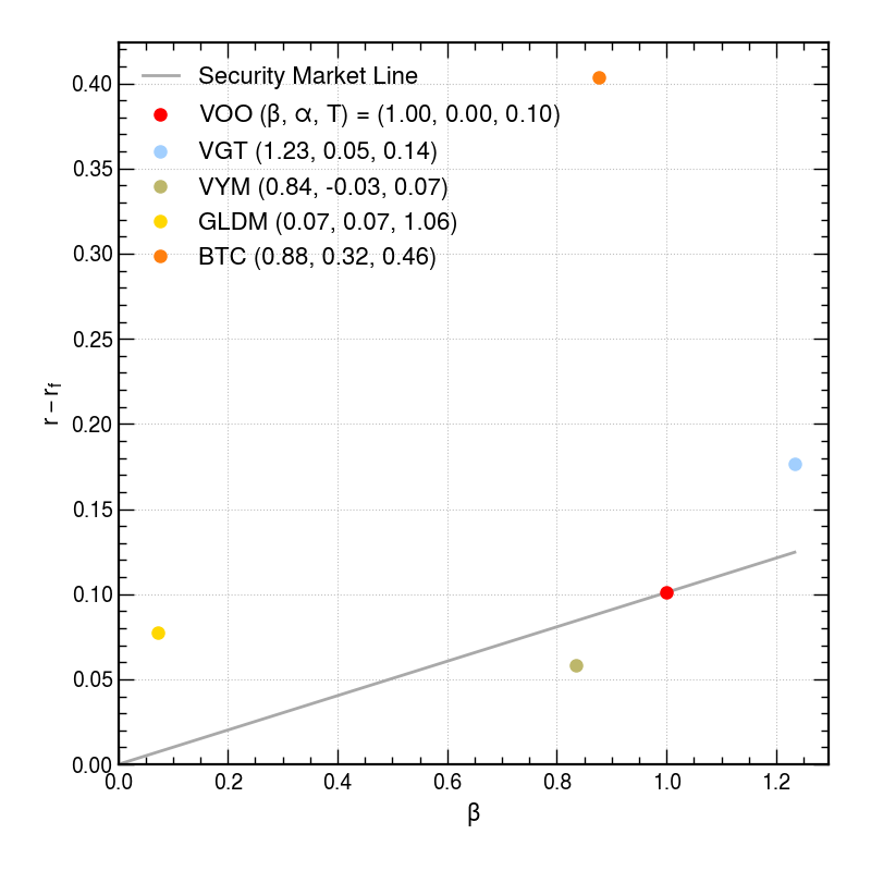
Assuming the simple form of the CAPM, the SML gives the predicted return of an asset with a given \(\beta\), and assuming \(\alpha = 0\). The \(\alpha\) of an asset shows how much it outperformed above this line.
More:
- Gibbons, M., Ross, S., & Shanken, J. (1989). A test of the efficiency of a given portfolio. 36
- Luenberger, D.G. (1998). Investment Science. 37
4.5 Factor models
4.5.1 Fama-French model
- Fama-French model three-factor model
- Fama, E.F. & MacBeth, J.D. (1973). Risk, return, and equilibrium: Empirical tests. 38
- Fama, E.F. & French, K.R. (1992). The cross-section of expected stock returns. 39
- Fama, E.F. & French, K.R. (2015). A five-factor asset pricing model. 40
- Yontar, T. & Benham, F. (2016). US small cap equity: Which benchmark is best?. 41
- Fama, E.F. & French, K.R. (2017). International tests of a five-factor asset pricing model. 42
38 Fama & MacBeth (1973).
39 Fama & French (1992).
40 Fama & French (2015).
41 Yontar & Benham (2016).
42 Fama & French (2017).
Three-factor model:
\[ r_{it} - r_{\mathrm{f}t} = \alpha_{i} + \beta^\mathrm{m}_{i} \, (r_{\mathrm{m}t} - r_{\mathrm{f}t}) + \beta^\mathrm{s}_{i} \, \mathrm{SMB}_{t} + \beta^\mathrm{v}_{i} \, \mathrm{HML}_{t} + \varepsilon_{it} \]
Five-factor model:
\[ r_{it} - r_{\mathrm{f}t} = \alpha_{i} + \beta^\mathrm{m}_{i} \, (r_{\mathrm{m}t} - r_{\mathrm{f}t}) + \beta^\mathrm{s}_{i} \, \mathrm{SMB}_{t} + \beta^\mathrm{v}_{i} \, \mathrm{HML}_{t} + \beta^\mathrm{p}_{i} \, \mathrm{RMW}_{t} + \beta^\mathrm{i}_{i} \, \mathrm{CMA}_{t} + \varepsilon_{it} \]
- \(r_\mathrm{m} - r_\mathrm{f}\): The return spread between the capitalization weighted stock market and cash.
- SMB: The return spread of small minus large stocks (i.e., the size effect).
- HML: The return spread of cheap minus expensive stocks (i.e., the value effect).
- RMW: The return spread of the most profitable firms minus the least profitable.
- CMA: The return spread of firms that invest conservatively minus aggressively. 43
43 Asness (2014).
4.5.2 Carhart four-factor model
- Carhart four-factor model
- Carhart, M.M. (1997). On persistence in mutual fund performance. 44
44 Carhart (1997).
Four-factor model:
\[ r_{it} - r_{\mathrm{f}t} = \alpha_{i} + \beta^\mathrm{m}_{i} \, (r_{\mathrm{m}t} - r_{\mathrm{f}t}) + \beta^\mathrm{s}_{i} \, \mathrm{SMB}_{t} + \beta^\mathrm{v}_{i} \, \mathrm{HML}_{t} + \beta^\mathrm{mom}_{i} \, \mathrm{PR1YR}_{t} + \varepsilon_{it} \]
On using momentum:
- Jegadeesh, N. & Titman, S. (1993). Returns to buying winners and selling losers: Implications for stock market efficiency. 45
45 Jegadeesh & Titman (1993).
4.5.3 Asness six-factor model
- Asness, C.S. & Frazzini, A. (2013). The Devil in HML’s Details. 46
- Asness, C.S. (2014). Our model goes to six and saves value from redundancy along the way. 47
- Asness, C.S., Frazzini, A., & Pedersen, L.H. (2019). Quality minus junk. 48
Six-factor model:
\[ r_{it} - r_{\mathrm{f}t} = \alpha_{i} + \beta^\mathrm{m}_{i} \, (r_{\mathrm{m}t} - r_{\mathrm{f}t}) + \beta^\mathrm{s}_{i} \, \mathrm{SMB}_{t} + \beta^\mathrm{v}_{i} \, \mathrm{HML}_{t} + \beta^\mathrm{p}_{i} \, \mathrm{RMW}_{t} + \beta^\mathrm{i}_{i} \, \mathrm{CMA}_{t} + \beta^\mathrm{mom}_{i} \, \mathrm{UMD}_{t} + \varepsilon_{it} \]
4.5.4 General factor analysis
- Factor analysis
- Fidelity. (2016). Putting factors to work.
- Fidelity. (2016). An overview of factor investing.
\[ r_{it} - r_{\mathrm{f}t} = \alpha_{i} + \sum_{j} \beta_{ij} \, f_{jt} + \varepsilon_{it} \]
- Regression with historical data gives \(\hat{\alpha}_{i}\) and \(\hat{\beta}_{ij}\).
- \(\beta_{ij}\) is called the factor loading or factor sensitivity for factor \(j\).
- Estimate the factor premiums, \(\hat{f}_{j}\), usually from historical return: \(\hat{f}_{j} = \mathbb{E}_{t}(f_{jt})\).
- Expected return: \(\hat{r}_{i} = \bar{r}_\mathrm{f} + \sum_{j} \hat{\beta}_{ij} \, \hat{f}_{j}\), where looking forward, it is usually assumed that \(\alpha_{i} = 0\).
It can be shown from OLS that
\[ \big[ \hat{\beta}^{\intercal} \big]_{ji} = \sum_k \big[ \mathrm{cov}(\vec{f}, \vec{f})^{-1} \big]_{jk} \, \big[ \mathrm{cov}(\vec{f}, \vec{r}) \big]_{ki} \]
The \(\beta\) vector over factors can be calculated for each asset independently.
\[ \hat{\vec{\beta}}_{i} = \mathrm{cov}(\vec{f}, \vec{f})^{-1} \cdot \mathrm{cov}(\vec{f}, r_{i}) \]
In the simple case of CAPM, there is a single factor, \(f_\mathrm{m} = r_\mathrm{m} - r_\mathrm{f}\).
4.6 Black-Litterman model
- Black-Litterman model
- Black, F. & Litterman, R. (1991). Asset allocation.49
- Black, F. & Litterman, R. (1992). Global portfolio optimization. 50
- He, G. & Litterman, R. (2002). The intuition behind Black-Litterman model portfolios. 51
- Meucci, A. (2008). The Black-Litterman approach: Original model and extensions. 52
4.7 Risk preferences
- Risk preferences
- Kelly criterion
- Kelly, J.L. (1956). A new interpretation of information rate. 53
- General consumption/investment problem
- Gambler’s ruin problem
- Merton’s portfolio problem
- Merton, R.C. (1969). Lifetime portfolio selection under uncertainty: The continuous-time case. 54
- Karatzas, I., Lehoczky, J.P., Sethi, S.P., & Shreve, S.E (1986). Explicit solution of a general consumption/investment problem. 55
- Conditional Value at Risk (CVaR) or Expected shortfall
- Rockafellar, R.T. & Uryasev, S. (2000). Optimization of conditional value-at-risk. 56
- Life-cycle strategy
- Modigliani, F. & Brumberg, R. (1954). Utility analysis and the consumption function: An interpretation of cross-section data. 57
- Scott, J.S., Shoven, J.B., Slavov, S.N. & Watson, J.G. (2023). The life-cycle model implies that most young people should not save for retirement. 58
- Anarkulova, A., Cederburg, S., & O’Doherty, M.S. (2025). Beyond the status quo: A critical assessment of lifecycle investment advice. 59
4.8 Postmodern portfolio theory
4.8.1 Criticisms of MPT
Criticisms of MPT:
- Sensitivity of portfolio weights to the estimates of \(\hat{\mu}\) and \(\hat{V}\).
- Uncertainty estimation; Error propagation
- Even assuming Gaussian distributed returns
- Variance is not a good measure of risk
- Downside risk is better
- Problem of induction
- Past performance is no guarantee of future results
- Criticisms of using historical estimators of \(\hat{\mu}\) and \(\hat{V}\)
- Non-Gaussian distributed returns
- Heteroskedasticity
- Criticisms of the Efficient Market Hypothesis
- To what degree are markets efficient?
4.8.2 Uncertainty estimation
- Error propagation; resampling the efficieny frontier
- Michaud, R.O. (1989). The Markowitz optimization enigma: Is ‘optimized’ optimal? 60
- Michaud, R.O. & Michaud, R.O. (2008). Efficient Asset Management. 61
- Lo, A.W. (2002). The statistics of Sharpe ratios. 62
- Bodnar, T. & Schmid, W. (2011). On the exact distribution of the estimated expected utility portfolio weights: Theory and applications. 63
- Bodnar, T., Mazur, S., & Podgórski, K. (2016). Singular inverse Wishart distribution and its application to portfolio theory. 64
- Becker, Y, Halffmann, P., & Schöbel, A. (2024). Risk management in multi-objective portfolio optimization under uncertainty. 65
- Fransisca, D.C., Sukono, Chaerani, D., & Halim, N.A. (2024). Robust portfolio mean-variance optimization for capital allocation in stock investment using the genetic algorithm: A systematic literature review. 66
- Kristensen, L. & Vorobets, A. (2024). Portfolio optimization and parameter uncertainty. 67
- Oliveira, D.C., Guzman, G., & Firoozye, N. (2025). (Non-parametric) bootstrap robust optimization for portfolios and trading strategies. 68
4.8.3 Downside risk
- Downside risk, semi-variance, semi-deviation, target semi-variance (TSV), target semi-deviation
- Estrada, J. (2000). The cost of equity in emerging markets: A downside risk approach. 69
- Estrada, J. (2002). Systematic risk in emerging markets: The D-CAPM. 70
- Estrada, J. (2008). Mean-semivariance optimization: A heuristic approach. 71
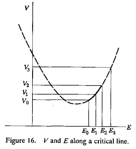
- Markowitz, H.M., Starer, D., Fram, H., & Gerber, S. (2019). Avoiding the downside: A practical review of the Critical Line Algorithm for mean-semivariance portfolio optimization. 72
- Mean-Semivariance frontier in scikit-portfolio
\[ \mathrm{TSV}(r_i, r_\mathrm{tan}) = \mathbb{E}\left[ (r_i - r_\mathrm{tan})^2 \: \mathbb{1}_{\{r_i < r_\mathrm{tan}\}} \right] \label{eq:target_semi_variance} \]
\[ \mathrm{TSD}(r_i, r_\mathrm{tan}) = \sqrt{\mathrm{TSV}(r_i, r_\mathrm{tan})} \label{eq:target_semi_deviation} \]
4.8.4 Heteroskedasticity
4.8.5 Criticisms of the efficient market hypothesis
- Bessembinder, H. & Chan, K. (1998). Market efficiency and the returns to technical analysis. 73
- Asness, C.S. (2024). The less-efficient market hypothesis. 74
- TODO: Room for fundamentally-motivated indicator analysis — sits between fundamental analysis and technical analysis.
See also:
4.8.6 More
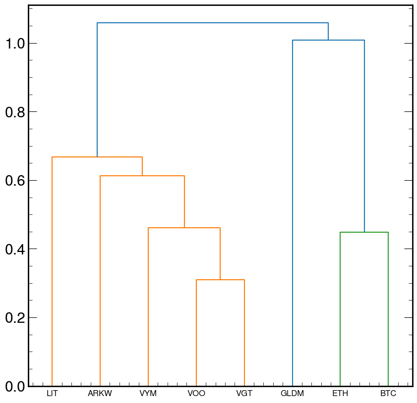
4.9 Hierarchical risk analysis
- Asset trees
- Stock correlation network
- Mantegna, R.N. (1998). Hierarchical structure in financial markets. 78
- Onnela, J.P., Chakraborti, A., Kaski, K., Kertész, J., & Kanto, A. (2003). Dynamics of market correlations: Taxonomy and portfolio analysis. 79
- Onnela, J.P., Kaski, K., & Kertész, J. (2004). Clustering and information in correlation based financial networks. 80
- Hierarchical Risk Parity (HRP)
- López de Prado, M. (2016). Building diversified portfolios that outperform out-of-sample. 81
- López de Prado, M. (2018). Advances in Financial Machine Learning. 82
- Lohre, H., Rother, C., & Schäfer, K.A. (2020). Hierarchical Risk Parity: Accounting for tail dependencies in multi-asset multi-factor allocations. 83
- Raffinot, T. (2018). Hierarchical clustering-based asset allocation. (HCAA) 84
- Raffinot, T. (2018). The hierarchical equal risk contribution portfolio. (HERC) 85
- Hudson & Thames. (2024). The Modern Guide to Portfolio Optimization. 86
- Cotton, P. (2024). Hierarchical minimum variance portfolios: A unifying approach using Schur complements. 87
- Blogs:
78 Mantegna (1998).
79 Onnela, J.P. et al. (2003).
80 Onnela, Kaski, & Kertész (2004).
81 López de Prado (2016).
82 López de Prado (2018).
83 Lohre, Rother, & Schäfer (2020).
84 Raffinot (2018a).
85 Raffinot (2018b).
86 Hudson & Thames (2024).
87 Cotton (2024).
Correlation distance between two assets:
\[ d_{ij} = \sqrt{\frac{1}{2} \left( 1 - \rho_{ij} \right)} \label{eq:hrp_distance} \]
Euclidean distance between two assets in \(n\)-assest space:
\[ \tilde{d}_{ij} = \sqrt{ \sum_{k=1}^{n} \left( d_{ki} - d_{kj} \right)^{2} } \label{eq:hrp_tilde_distance} \]
Note that \(\tilde{d}_{ij}\) is a function of the entire correlation matrix over all assets, whereas \(d_{ij}\) is defined for asset pairs.
4.10 Forecasting
This is the subject of Chapter 7.